Quantcast
Channel: ClearPeaks

How to Choose the Right Big Data Platform for Your Business

$
0
0

What are Your Requirements?


The very first question these days when it comes to the infrastructure for an organisation’s data platform, regardless of the architecture/paradigm being implemented (Data Warehouse, Data Lake, Data Lakehouse, Data Mesh, etc.), is basically – on-prem or cloud? But before considering that, it’s important to get the requirements from the business.


What are we trying to achieve, what is this data platform going to be used for? High-level architecture or paradigm? What are the business problems that we are trying to solve? Are the business stakeholders educated on the possibilities of data? Do they understand what sort of things are possible and what sort of things are not possible? Or if they are possible, do they have an indication of how expensive that is in terms of time, money, and effort? Asking the right questions is crucial here.


Of course,  it’s not possible to get all the requirements at once, but as I said before, if you can’t get the sample of these requirements, at least get the most important driving use cases.


On-Prem or Cloud?


Once we have the requirements as clear as possible, we can go back to the first question – the choice between cloud or on-prem. In general, the cloud offers many benefits – there is no large upfront investment, there is scalability, you don’t need to guess the required capacity of your platform, you just grow it with one click as you need.


Then there’s the availability of the clouds – in one click, you have a machine. And by availability, I also mean geographical availability. If you have a service running in the US and want to expand, in two clicks, you can have a service running in Australia or Asia.


We can also talk about the economies of scale. The cost per computer decreases the more computers you have, and of course one cannot compete in on-prem with the economies of scale that Amazon has, for instance.


There are also a lot of common showstoppers when organisations are trying to decide between cloud or on-prem, and I would say that there are two most common showstoppers. One is location. There are companies that say, “No, I cannot have my data off-prem or outside of our country.”


Of course, cloud vendors are aware of these concerns, and they are trying to address them now. Regarding the data location, the first thing they are trying to do is basically to bring their data centres to a larger number of physical locations, and in some cases, you can even have parts of AWS or Azure services on-prem.


The second major concern is about security – is the cloud secure? For this, I always respond with something that might sound a bit funny – can you imagine the amount of money and intelligence that giants like Amazon, Google, Oracle, and Microsoft invest into security issues?


Cloud platforms are secure – as long as you use them wisely, of course. If you have a cloud service, but you are using it unwisely and without proper governance and processes, then of course you can get into big problems, but if you know how to use cloud services and you use them well, they are as secure as an on-prem deployment.


Cloud Platforms


If, after consideration, you decide to choose a big data platform on the cloud, the next step is to choose a cloud provider. The four main contenders are AWS, Azure, GCP, and Oracle Cloud.


Traditionally, AWS is the market leader, though it seems like the competitors get a bit closer every year. When we look at the AWS offerings (and those of the rest), we have services to do almost all the things you can imagine of the data life cycle. For a few things, though, you may need help from external tools or services, which we will cover later on.


In AWS, the approach they take is kind of like Lego pieces. You can think of the different AWS services as Lego pieces; and to build a platform, you may need to put a lot of these pieces together. This requires a certain level of IT strength to implement.


On the other hand, Azure, which is, I would say, the most direct competitor of AWS, the services they have to build a data platform are easier to use, and normally you don’t require so many “Lego pieces”.


In an Amazon data platform, you may easily need 15 different types of services to do something. In Azure, maybe you need three or four different services. From a logical point of view, it’s usually easier to understand the logical structure of an Azure platform. Of course, that kills a bit of the flexibility.


So there is a trade-off – the more granular your Lego piece is, the more flexible you are. I’m not saying AWS is better or worse than Azure. It depends on your team, and on what you want to achieve.


The other main providers that we have in the picture, at least at ClearPeaks, are Oracle Cloud and GCP. GCP is pushing very hard and doing things very well. We have actually implemented GCP projects lately for some customers because of finding something in GCP that is just better and easier than the rest. So they are still not at the market leadership level of Azure, or AWS, but they are getting there.


Then we have the Oracle Cloud which is a great fit for Oracle customers that like Oracle’s robustness and Oracle products and services. Their offering is everyday more mature than the previous day. And likewise, we have recommended Oracle cloud to some customers, because we found that it made sense for the requirements of that situation.


When we talk about data and data platforms, there are a few other companies on our radar; which are Cloudera, Snowflake, Databricks, and Dremio. Those companies also have offerings to run on cloud.


We use Cloudera a lot with our customers. On the on-prem, as I will say later, they are unrivalled. And when it comes to the cloud, especially when you want to deal with multi clouds, with hybrid things like cloud and on-prem, or when your required workloads are very varied, then Cloudera becomes the best option.


Snowflake is a cloud data warehouse. If you need a data warehouse in the cloud, Snowflake is probably one of the best options out there. They are trying to win market share by trying to expand the scope of the services they offer, aiming  at a data lakehouse and including streaming, machine learning, and more.


Databricks was started by the same people that created Spark, so it has the best Spark you can find. And like Snowflake, Databricks is also trying to evolve the scope of what it offers, from having just the best Spark on cloud to creating a data lakehouse with Delta Lake technologies and making a lot of investment on offerings related to machine learning and artificial intelligence.


Dremio is also positioned as a lakehouse platform and offers quite a few different approaches compared to other technologies. It has recently released a pure SaaS (Software as a Service) offering so it is also starting to be a mature alternative.


So between AWS, Azure, GCP, Oracle Cloud, Cloudera, Snowflake, Databricks and Dremio, I would say that more than 90% of your needs are covered. There still maybe some cases that you may need support.


When you think about the internal part of the data platform, you are more than covered with all these providers, but when you think about the peripheral areas of the data platform like data ingestion, orchestration, CI/CD, automation, governance, federation and virtualisation, or visualisation, you may need something more.


For example, AWS, Azure, and other providers are fine with ingesting data between their services. But if you want to ingest data from outside, they are not as good, and you may need a tool for ingestion specifically. Then you have some nice platforms out there like Informatica or Talend, which not only deal with ingestion, but they also allow you to do orchestration, governance, and other things in one single platform.


Then onto visualisation – again, most of the providers I’ve mentioned have visualisation services, but they are maybe lacking the robustness of other technologies that have been serving as visualisation layers for many years, such as Tableau. This is why we often see Tableau in tandem with these technologies.


On-Prem Deployments


If an organisation wants on-prem, that may not only be because of security concerns, or like I said before, the data location. There is a third reason for staying on-prem, and I have recommended it myself sometimes. If you know exactly what you need and how big you are, and you have the team that knows how to do it, on-prem is the best option. In this case, it’s going to be cheaper to be on-prem in the long-term.


We’ve done that study with one of our customers. They wanted a platform, and they knew perfectly what they wanted. So we could size it accurately and make a good comparison. What we found out was that for this particular customer, cloud was cheaper in the beginning of course, because for on-prem you had to buy the equipment.


But then we also tried to estimate the demand, effort, and all the other variables. Through this analysis and estimation, we found that if the platform was going to be 100% utilised, over five years, the on-prem was going to be cheaper than the cloud. For the first four years, cloud was going to be cheaper, but after five years, the on-prem started to be the cheaper option.


Then at this point, you can wonder – in five years, is the platform really going to be doing what I want to do at that point? Probably not.  But still, my point is that there are still some situations in which the requirements, forgetting about data location and security, may still make it a sensible choice to stay on-prem.


After making the decision to go for an on-prem deployment, we need to think about what tool stacks are available. Our preferred contenders are the ones we have mentioned in this article – but there are many more technologies out there!


There is also an increase of the open-source movement, so you can see data platforms with stuff like PostgreSQL, MySQL, Superset, a lot of Python and R for the machine learning use cases, Airflow for orchestration, etc. Some of these traditional open-source tools like Airflow, for example, are now becoming integrated into the clouds. Amazon just released a managed Airflow, and Google has already had it for a while. So we’re seeing some interesting movements now in this space.


Private Cloud


There are two flavours in on-prem – bare-metal, in which you install what you need directly on the machine; or you have a virtualisation layer that sits on top of bare-metal, which is referred to as a private cloud.


In a private cloud, you basically have a bunch of virtual machines on which you install whatever you want. This virtualisation layer has a penalty in terms of efficiency. You always have better performance when you have whatever you want installed directly on your bare-metal machine, versus having a virtualisation layer. Having a virtualisation layer adds some overhead that makes things a bit slower, but it gives a lot of flexibility.


It’s very common to have private cloud deployments in on-prem, it gives you something similar to the IaaS (Infrastructure as a Service) that you get on the cloud. While concepts like PaaS (Platform as a Service) and SaaS have been limited to the cloud, this is changing a bit lately in the data world, thanks to Kubernetes, Docker, and the like. In Cloudera, for example, they have recently released something called the analytics experiences which allow you to have the kind of ephemeral experience you would get on a cloud, with on-prem. It is going to be more and more common to have these ephemeral experiences also with on-prem.


Consider the Cost


When we think about on-prem, it’s a given that it is more expensive than cloud because you need to have the infrastructure and the people to deploy and maintain your platform. But sometimes in cloud, there’s something that is a bit tricky to navigate. When one puts a data platform in the cloud, there is a change of mindset that one needs to have, which is basically, you always need to look at your pocket.


As Amazon will tell you, you pay for what you use. That can be as granular as paying per query. So if that query that you run is not efficient, you may be incurring a high cost that you don’t expect. It can run into thousands of Euros for a single accidental bad query. This means that whenever you’re developing something on the cloud, you always need to have this concern, which I would say is a bit less worrying in on-prem.


If you do a bad query on on-prem it’s not as catastrophic as it can be on the cloud. Of course, clouds have measures to help you prevent these mishaps. But they are measures that you need to always have in your mind, basically setting guard rails that prevent extra costs.


Conclusion


Whichever vendor and architecture you choose, the success or failure depends on how well it fulfils the business requirements. It’s important to always have a business-driven initiative in this case.


And of course, we are happy to help you get this clarity. We have these conversations regularly and would love to talk to you. Simply contact us!


Big Data and Cloud Services blog banner

The post How to Choose the Right Big Data Platform for Your Business appeared first on ClearPeaks.

Versioning NiFi Flows and Automating Their Deployment with NiFi Registry and NiFi Toolkit

$
0
0

When it comes to the efficient development of data flows, one can argue there should be a way to store different versions of the flows in some central repository and the possibility to deploy those versions in multiple environments, just as we would do with any piece of code for any other software.


In the context of Cloudera Data Flow, we can do so thanks to Cloudera Flow Management,  powered by Apache NiFi and NiFi Registry, and NiFi Toolkit, which we can use to deploy flow versions across NiFi instances from different environments integrated with NiFi Registry.


In this article, we will demonstrate how to do this, showing you how to version your NiFi flows using NiFi Registry and how to automate their deployment by combining shell scripts and NiFi Toolkit commands.


1. Introduction


Apache NiFi is a robust and scalable solution to automate data movement and transformation across various systems. NiFi Registry, a subproject of Apache NiFi, is a service which enables the sharing of NiFi resources across different environments. Resources, in this case, are data flows with all their properties, relationships and processor configurations, but versioned and stored in Buckets – containers holding all the different versions and changes made to the flow. In other words, it enables data flow versioning in Git style. Just like versioning the code; we can commit local changes, revert them, and pull and push versions of the flows. It also offers the possibility to store versioned flows to external persistence storage, like a database.


Generally speaking, there are two possible scenarios when you would use NiFi Registry in your organisation. The first  is to have one central service shared across different environments, and the second  is to have one NiFi Registry service per environment.


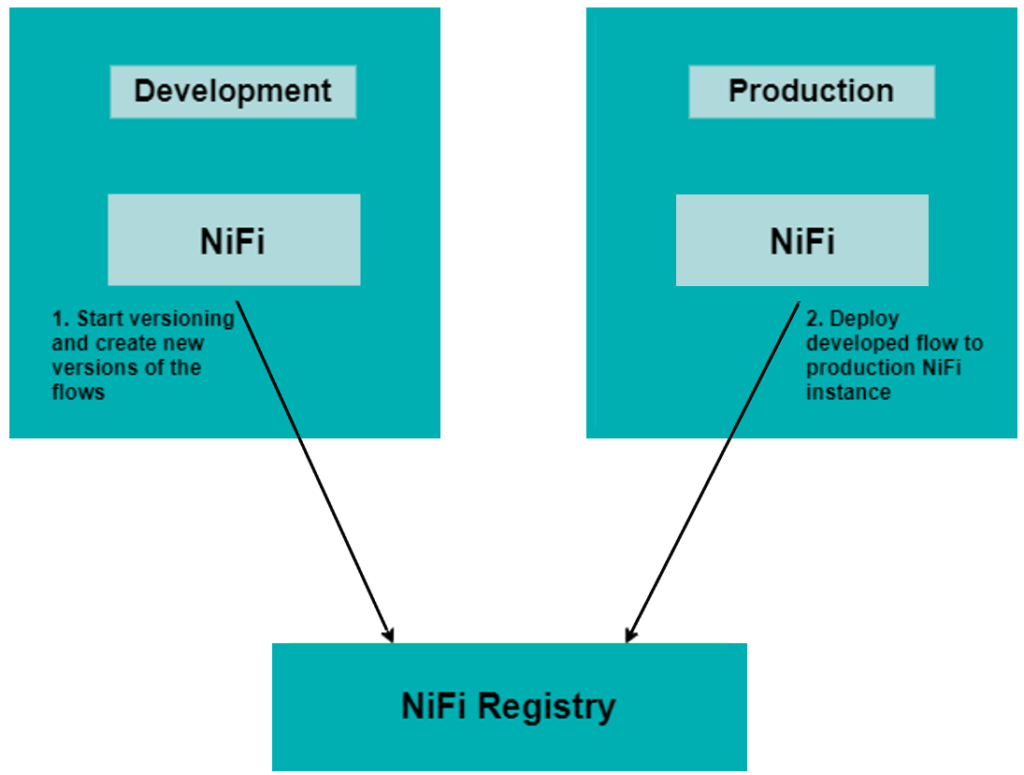
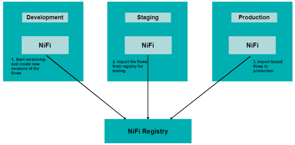
In the picture below we can see a representation of the first scenario: one NiFi Registry is used as the central instance and flows can be shared across different environments during or after their development. This is a common situation, in which we can create the flows in Development, push them to NiFi Registry in the form of multiple versions, pull them to the Staging area to conduct some tests after reaching some milestones, and eventually push them to Production once we are satisfied with the flow behaviour.


NiFi Registry deployment scenario 1

Figure 1: NiFi Registry deployment scenario  1


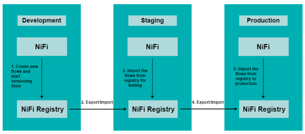
In the second scenario, depicted below, we have one NiFi Registry per environment: in this case, we can develop the desired flow in one environment, and when the flow is ready for the next logical environment, we can export it from one NiFi Registry instance and import it to the next one.


This requires more steps in comparison with the first deployment scenario, but sometimes companies have very restricted and isolated environments which cannot communicate with each other for security reasons. In such a case, this is a good option to have versioned flows and to control their development life cycle.


NiFi Registry deployment scenario 2

Figure 2: NiFi Registry deployment scenario 2


The flow migration  between different NiFi Registry instances requires NiFi Toolkit commands. NiFi Toolkit is very popular among data flow administrators and NiFi cluster administrators, because it provides an easy way to operate the cluster and the data flows. It is a set of tools which enables the automation of tasks such as flow deployment, process groups control and cluster node operations. It also provides a command line interface (CLI) to conduct these operations interactively (you can check out more details about it at this link).


NiFi Toolkit can also be used  to migrate the flows between NiFi instances in the same security areas with connectivity between them, as in scenario 1 described above. In this article, we will use NiFi Toolkit to migrate the flows using one common NiFi Registry integrated with two NiFi instances.


2. Demo Environment


For this demonstration, we are reproducing a simplified version of the first scenario  described above, using two NiFi instances running on the same machine and integrated with one NiFi Registry service, all running on Linux Ubuntu server 20.04 LTS.


Demo environment architecture

Figure 3: Demo environment architecture


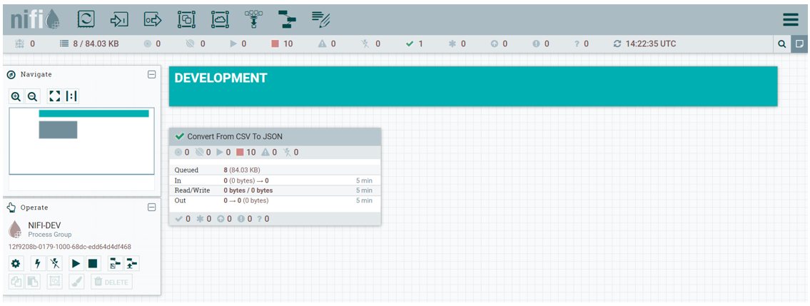
One NiFi instance runs on port 8080 and  is used as the Development environment (see this link for details on how to install and run NiFi on your local machine is described). In this environment, we created a simple data flow which transforms CSV data to JSON format data.


Development NiFi instance

Figure 4: Development NiFi instance


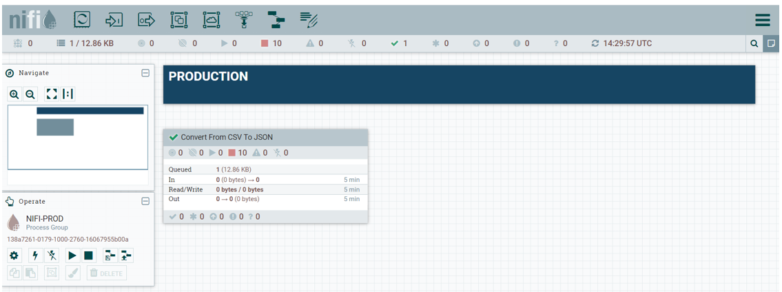
Another NiFi instance is used as the Production environment, running on port 8081. This instance is the final target instance to which we will be pushing all the flows that have the desired behaviour and tested logic. In our scenario, to make it simpler, we do not have a staging area for testing, but the deployment procedure that will be shown in this article is the same.


Production NiFi instance

Figure 5: Production NiFi instance


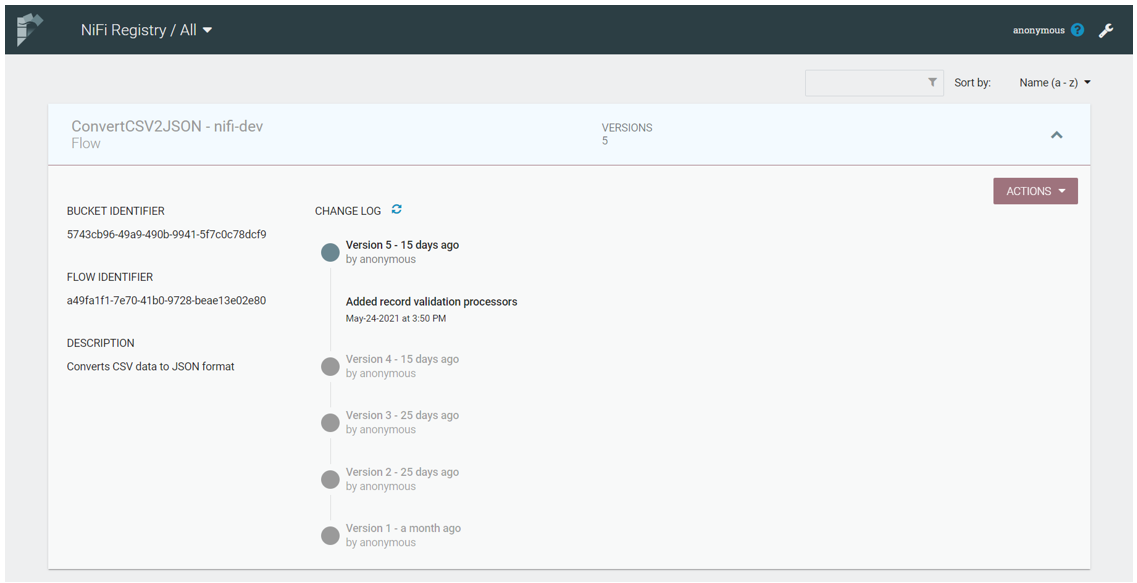
The NiFi Registry instance is running on the same server, on port 18080. The interface is much simpler than the NiFi UI, as you can see below:


NiFi Registry UI

Figure 6: NiFi Registry UI


In the above picture, you can see one NiFi Registry bucket called “nifi-dev” and one versioned flow called “ConvertCSV2JSON”. The same flow has 5 versions, which we can see listed from the most recent to the oldest. If we click on each version, the commit comment will be shown. If required, we can add more buckets and separate versions of the flow, according to, for example, some milestones in the development. Note that NiFi Registry stores flows at the level of a Processor Group on the NiFi canvas: it cannot store only one independent component of the flow (like, for example, a single processor).


NiFi Registry can also be configured to push versions of the flow to GitHub automatically every time a commit is done from the NiFi canvas. This section of the NiFi Registry documentation describes how to add GitHub as a flow persistence provider.


3. NiFi Flow Versioning


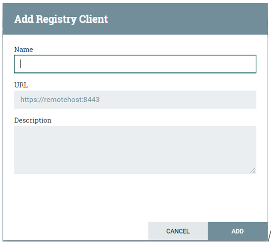
To be able to store different versions of the flow in the Development environment, the NiFi instance needs to be connected to the NiFi Registry service. To connect NiFi to NiFi Registry, go to the upper right corner of the NiFi taskbar and select the little “hamburger” menu button. Then, select “Controller setting” and the “Registry clients” tab. There, click on the upper right + symbol to add a new Registry client.


Adding a new Registry client

Figure 7: Adding a new Registry client


In the next window, we have to specify the Registry name and URL; optionally we can add a description.


Adding Registry client details

Figure 8: Adding Registry client details


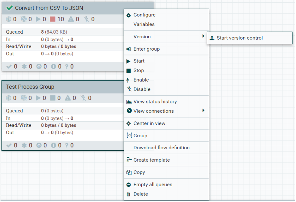
To be able to version the flows after making some changes, you need to start version control for that Processor Group. To do so, right-click on the desired Processor Group, select “Version”, and click on “Start version control”.


Start flow version control

Figure 9: Start flow version control


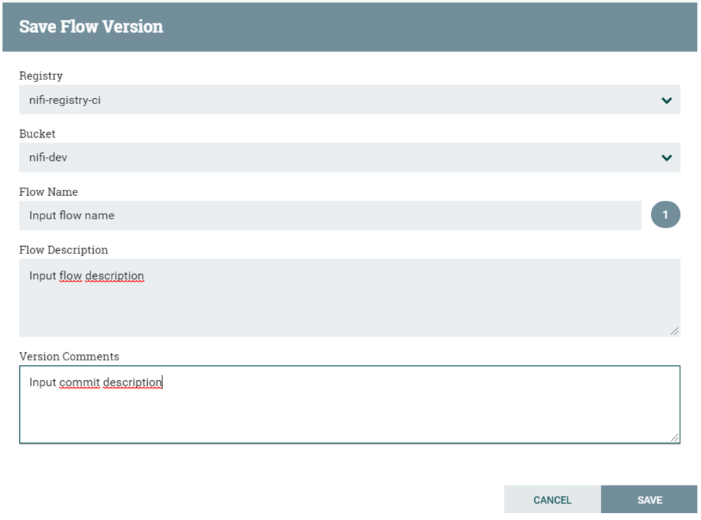
In the following window, select the desired NiFi Registry instance, select the bucket, and specify the flow name, the flow description and the commit message with a description of the changes.


Flow version commit details

Figure 10: Flow version commit details


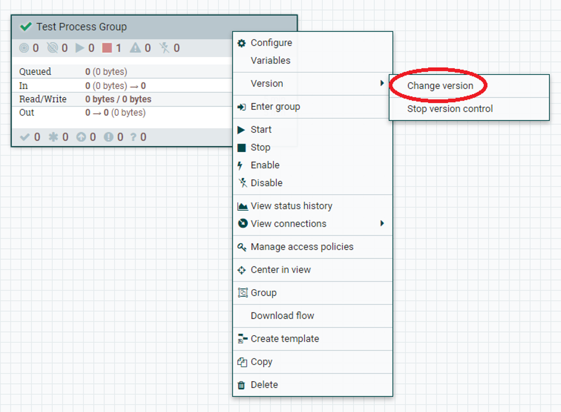
In this way, the current version of the Processor Group is saved as the initial version in the NiFi Registry bucket with its corresponding commit message. As the development of the flow progresses, you will create new versions, but you will always be able to roll back to a previous version if required. To do this, right-click on the desired Processor Group, go to “Version” and then to “Change version”.


Changing the flow version

Figure 11: Changing the flow version


A window like the one below will open, where we can select the desired version of the flow to which we want to roll back.  There are also comment details for each version, so it is always a good idea to add some meaningful comments to every commit to help you later when rolling back.


Saved flow versions list

Figure 12: Saved flow versions list


You can also list or revert local changes before they are committed: after changes have been made in the Processor Group, in the upper left corner there will be a * symbol, which indicates there are uncommitted changes in this Processor Group. After they have been committed, the symbol changes to a green . To list local changes or to revert them, right-click on the desired Processor Group and then go to “Version”. After that, depending on the need, select either “Show local changes” or “Revert local changes”, as shown below:


Local changes actions

Figure 13: Local changes actions


4. NiFi Flow Deployment without a common NiFi Registry


What we have described in the above sections relates to scenarios in which we have a central NiFi Registry that is shared between different environments. However, as we mentioned in the introduction, there may be situations in which, as seen in scenario 2, the various environments are isolated and cannot share a common NiFi Registry. For these cases we recommend applying the approach detailed below. Note that in this article, we are simulating a scenario with two NiFi instances and one NiFi Registry running on the same machine with connectivity between them; in real life this may not be the case. So before importing the exported files into the target environment, you will obviously have to move the files to a location with connectivity to the target environment.


4.1. Installing NiFi Toolkit


Nifi Toolkit can be downloaded from the Apache NiFi official page, in the Downloads section. At the time of writing, the most recent version is 1.13.2.

To download it, we use the “wget” command. This will download a .gzip archive to the desired folder; then we can extract the file using the “tar” tool and we can start the toolkit CLI, as shown below:


mkdir /etc/nifi-toolkit
cd /etc/nifi-toolkit
wget https://www.apache.org/dyn/closer.lua?path=/nifi/1.13.2/nifi-toolkit-1.13.2-bin.tar.gz
tar -xvf nifi-toolkit-1.13.2-bin.tar.gz
cd nifi-toolkit-1.13.2
./bin/cli.sh


The “help” command will list all possible commands which can be used inside the toolkit. In our case, we will be using the following:

  • nifi list-param-contexts
  • nifi export-param-contexts
  • nifi import-param-contexts
  • nifi merge-param-context
  • registry list-buckets
  • registry list-flows
  • nifi pg-import
  • nifi pg-change-version
  • nifi pg-enable-services
  • nifi pg-start

By typing “command-name help”, we can see the command description, its purpose and its possible options and arguments.


4.2. Migrating the parameter context


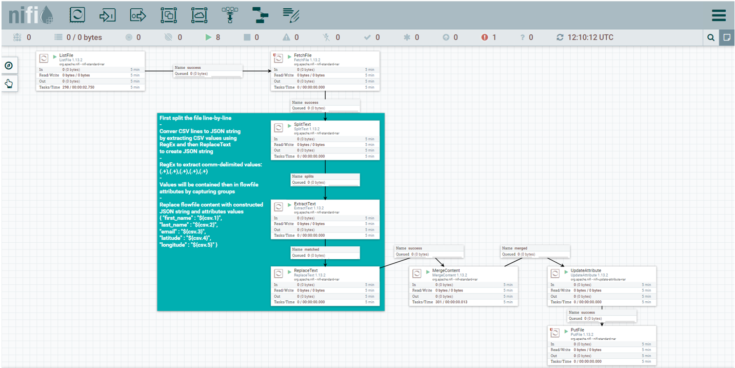
In our development NiFi instance, we have created a data flow which converts CSV data to JSON data and dumps the converted data file in a specific folder.


Development data flow

Figure 14: Development data flow


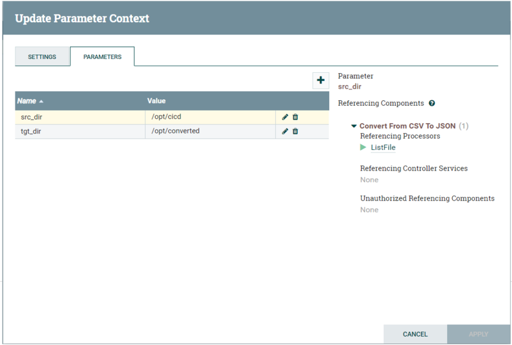
Source and target folders for the input CSV and output JSON files are specified in the parameter context of the NiFi flow.


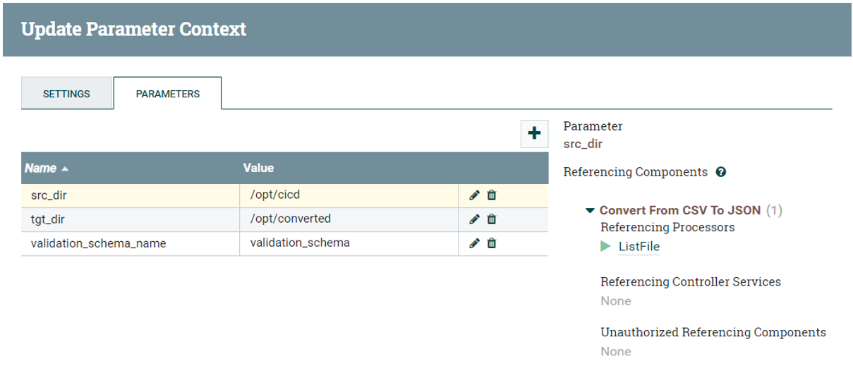
Parameter context

Figure 15: Parameter context


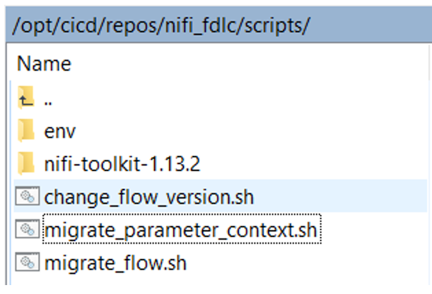
This is the first version of our flow, and we want to deploy it to the Production NiFi instance. As we said earlier, here we will use shell scripts combined with NiFi Toolkit. It is important to note that there needs to be a NiFi Toolkit folder with all its dependencies and libraries in the same folder as the deployment shell scripts. Moreover, there should also be an “env” folder containing property files for every NiFi instance we are using and for the NiFi Registry instance in the same folder.


The picture below shows the content of the folder for our demo (containing all the shell scripts we will describe in the following sections):


Folder structure with deployment scripts

Figure 16: Folder structure with deployment scripts


The property files in the /env folder enable NiFi Toolkit commands to know on which URL the target NiFi instances are running. An example of the property file for the Production NiFi instance is shown below:


baseUrl=http://192.168.1.8:8081
keystore=
keystoreType=
keystorePasswd=
keyPasswd=
truststore=
truststoreType=
truststorePasswd=
proxiedEntity=


In the Property file we can also specify the keystore and truststore file paths in case we have secured NiFi instances using SSL/TLS, but this is beyond the scope of this article.


To migrate our flow to the Production NiFi instance, we first need to migrate the parameter context which is used by the FetchFile and PutFile processors in the flow. To do so, we have developed the following shell script. Note that migrating the parameter context in this way is only necessary when we are not using a common NiFi Registry; only in that situation do we need to migrate the parameter context between NiFi Registries by using exported JSON files. However, it is an option even if we have scenario 1 with a common NiFi Registry as described above, but it is not mandatory.


#!/bin/bash

#Migrates parameter context from one environment to another
set -e #Exit if any command fails
output_file="$1"# Read agruments
src_env="$2"
tgt_env="$3"
#Set Global Defaults
[ -z "$FLOW_NAME" ] && FLOW_NAME="ConvertCSV2JSON"
case "$src_env" in
dev)
    SRC_PROPS="./env/nifi-dev.properties";;
*)
    echo "Usage: $(basename "$0")    "; exit 1;;
esac
case "$tgt_env" in
prod)
    TGT_PROPS="./env/nifi-prod.properties";;
*)
    echo "Usage: $(basename "$0")    "; exit 1;;
esac
echo "Migrating parameter context from '${FLOW_NAME}' to ${tgt_env}...."
echo "==============================================================="
echo -n "Listing parameter contexts from environment "$src_env"....."
param_context_id=$(./nifi-toolkit-1.13.2/bin/cli.sh nifi list-param-contexts 
-ot json -p "$SRC_PROPS" | jq '.parameterContexts[0].id')
echo "[\033[0;32mOK\033[0m]"
echo -n "Exporting parameter context from environemnt ${src_env}......"
./nifi-toolkit-1.13.2/bin/cli.sh nifi export-param-context -pcid ${param_context_id} 
-o ${output_file} -p "$SRC_PROPS" > /dev/null
echo "[\033[0;32mOK\033[0m]"
echo -n "Importing parameter context to environment ${tgt_env}........"
./nifi-toolkit-1.13.2/bin/cli.sh nifi import-param-context -i ${output_file} -p "$TGT_PROPS" > 
/dev/null
echo "[\033[0;32mOK\033[0m]"
echo "Migration of parameter context from ${src_env} to ${tgt_env} successfully finished!"
exit 0


This script is referencing the environment property files that we mentioned before. In total, it is using three arguments:

  • the path of the JSON export file with parameter context
  • the name of the Source environment
  • the name of the Production environment


The first step of the script lists the parameter contexts on the Development environment and saves the parameter context identifier in a local variable for later usage. This is done by the JSON command line tool “jq”, which we are using to mimic the backreferencing feature: in the interactive NiFi Toolkit mode, results of the previously typed commands can be referenced using the & character (as described here); in our case, however, since we are in a shell script, backreferencing is not possible, so we have to save the command results in JSON format in the local variable, and use them in the next command.


techo@ubuntu-dev:/opt/cicd/repos/nifi_fdlc/scripts$ sh migrate_parameter_context.sh 
/opt/cicd/repos/nifi_fdlc/scripts/env/dev_parameter_context.json dev prod
Migrating parameter context from 'ConvertCSV2JSON' to prod....
===============================================================
Listing parameter contexts from environment dev.....[OK]
Exporting parameter context from environment dev......[OK]
Importing parameter context to environment prod........[OK]

Migration of parameter context from dev to prod successfully finished!


Once the script is completed successfully, we can see that the parameter context has been imported to the Production NiFi environment.


Imported Parameter context in production NiFi instance

Figure 17: Imported Parameter context in production NiFi instance


4.3. Migrating the developed flow


After migrating the parameter context, we are ready to migrate our developed flow from the Development to the Production NiFi instance. To do so, we will use another shell script which includes some NiFi Toolkit commands for importing process groups from one instance to another. The requirement for this task is that both NiFi instances are integrated with the central NiFi Registry instance. The shell script for the migration has the following code:


#!/bin/bash

#Migrates flow from one environment to another
#Exit if any command fails
set -e
# Read agruments
version="$1"
target_env="$2"
#Set Global Defaults
[ -z "$FLOW_NAME" ] && FLOW_NAME="ConvertCSV2JSON"
case "$target_env" in
prod)
    PROD_PROPS="./env/nifi-prod.properties";;
*)
    echo "Usage: $(basename "$0")   "; exit 1;;
esac
echo "Migrating flow '${FLOW_NAME}' to environment ${target_env}"
echo "==============================================================="
echo -n "Listing NiFi registry buckets......"
bucket_id=$(./nifi-toolkit-1.13.2/bin/cli.sh registry list-buckets -ot json 
-p "./env/nifi-registry.properties" | jq '.[0].identifier')
echo "[\033[0;32mOK\033[0m]"
echo -n "Listing NiFi registry flows........"
flow_id=$(./nifi-toolkit-1.13.2/bin/cli.sh registry list-flows -b ${bucket_id} -ot json 
-p "./env/nifi-registry.properties" | jq '.[0].identifier')
echo "[\033[0;32mOK\033[0m]"
echo -n "Deploying flow ${FLOW_NAME} to environment ${target_env}......."
./nifi-toolkit-1.13.2/bin/cli.sh nifi pg-import -b ${bucket_id} -f ${flow_id} -fv ${version} 
-p "$PROD_PROPS" > /dev/null
echo "[\033[0;32mOK\033[0m]"
echo "Flow deployment to environment ${target_env} successfully finished!"
exit 0


This script is also using the property files from the /env folder to locate the URL on which NiFi Registry and the Production NiFi instances are running. It is using two arguments: the flow version number, and the name of the environment which the script uses to locate the property file and the required URL.


The first step in the script lists all the buckets from NiFi Registry and saves the bucket identifier in a local variable. In the following step, the script lists the flow identifier and saves it in a local variable for later usage. In the last step, the script uses the identifier from the previous step to find the flow in the NiFi Registry before importing it to the Production NiFi instance.


techo@ubuntu-dev:/opt/cicd/repos/nifi_fdlc/scripts$ sh migrate_flow.sh 6 prod
Migrating flow 'ConvertCSV2JSON' to environment prod
===============================================================
Listing NiFi registry buckets......[OK]
Listing NiFi registry flows........[OK]
Deploying flow ConvertCSV2JSON to environment prod.......[OK]
Flow deployment to environment prod successfully finished!


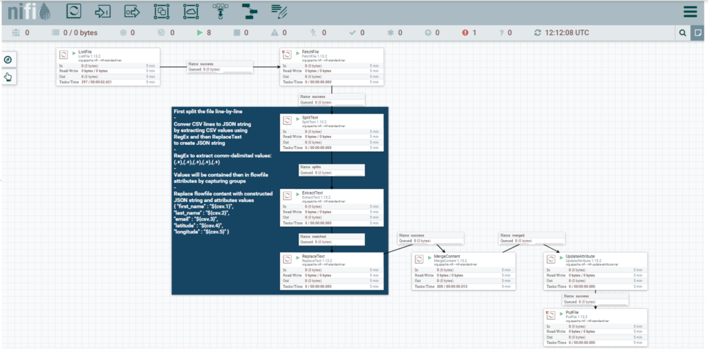
After the script execution is finished, we can see our flow has been deployed in the Production NiFi instance:


Deployed flow in production NiFi instance

Figure 18: Deployed flow in production NiFi instance


4.4. Changing the flow version live


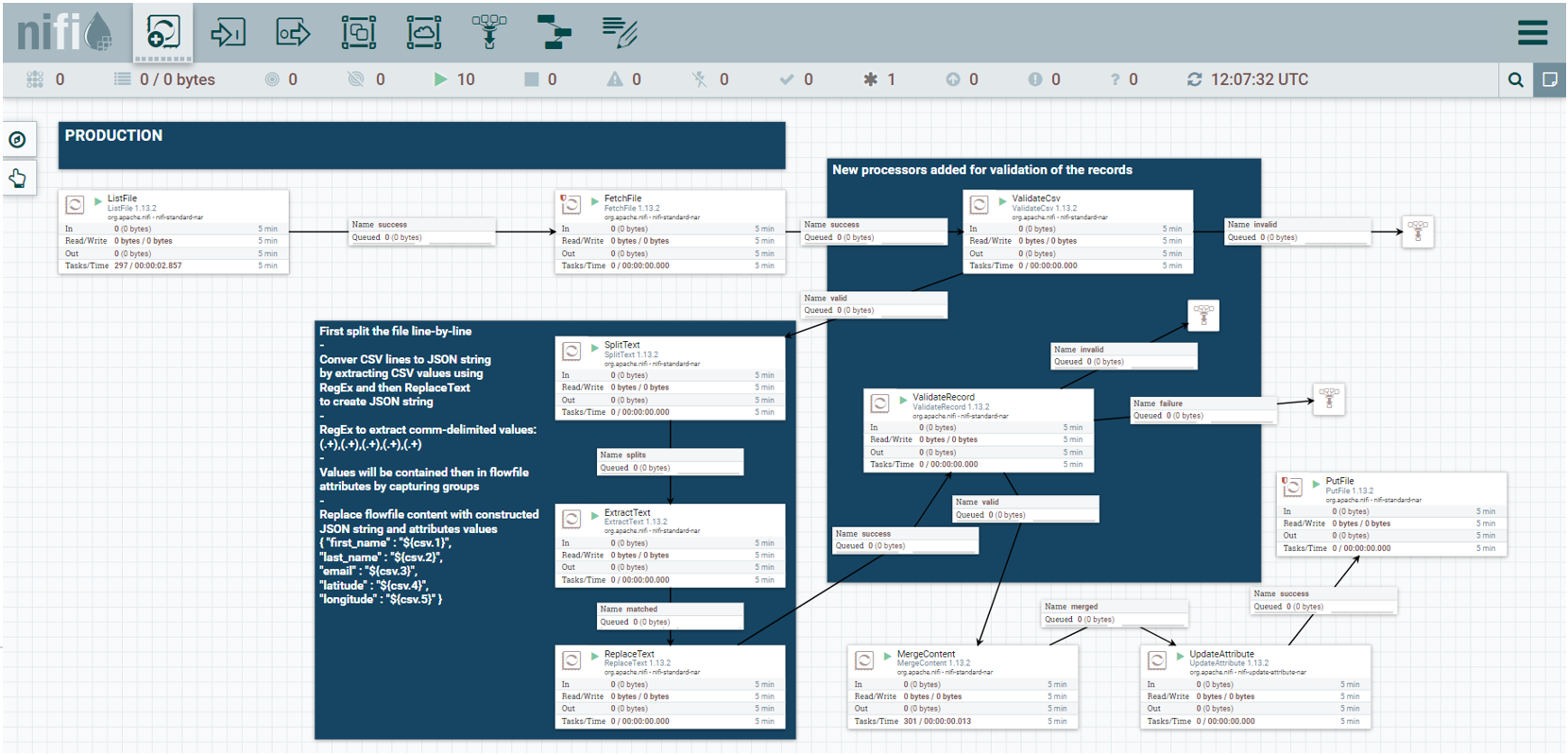
The flow is now deployed in the Production NiFi instance, and it is up and running. Let us now suppose that the business users realised that there are some invalid records in the CSV data coming in and out of the flow. These records are empty, having value “null” or just an empty string, so we need to introduce some data quality checks in our flow and develop a new version of it. After the development is finished, we want to migrate the flow to the Production environment, but we do not want to interfere with the existing flow which is already running, and maybe there is some data in the pipeline that we do not want to corrupt. To do so, we will use another shell script combined with NiFi Toolkit commands which will allow us to migrate the flow without risking such errors.


On the Development NiFi instance we have prepared the new version of the flow. It includes an updated parameter context (with a new parameter called “validation_schema_name”), two new processors to validate data records (“ValidateCsv” and “ValidateRecord”) and new Controller services to go along with them. All of these elements will be migrated to the Production NiFi instance.


First, we need to update the parameter context. This can be done using the NiFi Toolkit command for merging parameter contexts, as in the shell script shown below:


#!/bin/bash

#Merges parameter context from one environment with another
#Adds missing parameters from one environment that are missing
#in another environment

#Exit if any command fails
set -e
# Read agruments
output_file="$1"
src_env="$2"
tgt_env="$3"
pc_id="$4"
#Set Global Defaults
[ -z "$FLOW_NAME" ] && FLOW_NAME="ConvertCSV2JSON"
case "$src_env" in
dev)
    SRC_PROPS="./env/nifi-dev.properties";;
*)
    echo "Usage: $(basename "$0")     "; exit 1;;
esac
case "$tgt_env" in
prod)
    TGT_PROPS="./env/nifi-prod.properties";;
*)
    echo "Usage: $(basename "$0")    "; exit 1;;
esac
echo "Merging parameter context from '${FLOW_NAME}' to ${tgt_env}...."
echo "==============================================================="
echo -n "Listing parameter contexts from environment "$src_env"....."
param_context_id=$(./nifi-toolkit-1.13.2/bin/cli.sh nifi list-param-contexts -ot json 
-p "$SRC_PROPS" | jq '.parameterContexts[0].id')
echo "[\033[0;32mOK\033[0m]"
echo -n "Exporting parameter context from environment "${src_env}"......"
./nifi-toolkit-1.13.2/bin/cli.sh nifi export-param-context -pcid ${param_context_id} 
-o ${output_file} -p "$SRC_PROPS" > /dev/null
echo "[\033[0;32mOK\033[0m]"
echo -n "Merging parameter context to environment "${tgt_env}"........"
./nifi-toolkit-1.13.2/bin/cli.sh nifi merge-param-context -pcid ${pc_id} -i ${output_file} 
-p "$TGT_PROPS" > /dev/null
echo "[\033[0;32mOK\033[0m]"
echo "Merging parameter context from "${src_env}" with "${tgt_env}" successfully finished!"
exit 0


After the script has been successfully executed, we can see that the parameter context in the Production NiFi instance has the newly added parameter containing the validation schema name.


Merged parameter context in production NiFi

Figure 19: Merged parameter context in production NiFi


Now we can migrate the newly developed flow to the Production NiFi instance. To do so, we use another shell script. The first step implicitly disables all the services and controllers in the Production flow and changes the flow version to the desired new one; the second step re-enables all the services and controllers; the last step restarts the Processor Group to continue with the data flow.


#!/bin/bash

#Deploys development flow to target environment
#Exit if any command fails
set -e
# Read agruments
version="$1"
target_env="$2"
target_pgid="$3"
#Set Global Defaults
[ -z "$FLOW_NAME" ] && FLOW_NAME="ConvertCSV2JSON"
case "$target_env" in
dev)
    DEV_PROPS="./env/nifi-dev.properties";;
prod)
    PROD_PROPS="./env/nifi-prod.properties";;
*)
    echo "Usage: $(basename "$0")    "; exit 1;;
esac
echo "Deploying version ${version} of '${FLOW_NAME}' to ${target_env}"
echo "==============================================================="
echo -n "Checking current version..."
current_version=$(./nifi-toolkit-1.13.2/bin/cli.sh nifi pg-get-version -pgid "$target_pgid" -ot json 
-p "$PROD_PROPS" | jq '.versionControlInformation.version')
echo "[\033[0;32mOK\033[0m]"
echo "Flow ${FLOW_NAME} in ${target_env} is currently at version: ${current_version}"
echo -n "Deploying flow........."
./nifi-toolkit-1.13.2/bin/cli.sh nifi pg-change-version -pgid "$target_pgid" -fv $version 
-p "$PROD_PROPS" > /dev/null
echo "[\033[0;32mOK\033[0m]"
echo -n "Enabling services......"
./nifi-toolkit-1.13.2/bin/cli.sh nifi pg-enable-services -pgid "$target_pgid" -p "$PROD_PROPS" > /dev/null
echo "[\033[0;32mOK\033[0m]"
echo  -n "Starting process group...."
./nifi-toolkit-1.13.2/bin/cli.sh nifi pg-start -pgid "$target_pgid" -p "$PROD_PROPS" > /dev/null
echo "[\033[0;32mOK\033[0m]"
echo "Flow deployment successfully finished, ${target_env} is now at version ${version}!"
exit 0


After a successful execution, we can see that the updated flow has been deployed in the NiFi Production instance, and is running correctly.


techo@ubuntu-dev:/opt/cicd/repos/nifi_fdlc/scripts$ sh change_flow_version.sh 7 prod 
fa62a037-0179-1000-7075-953ab6326d53
Deploying version 7 of 'ConvertCSV2JSON' to prod
===============================================================
Checking current version...[OK]
Flow ConvertCSV2JSON in prod is currently at version: 6
Deploying flow.........[OK]
Enabling services......[OK]
Starting process group....[OK]
Flow deployment successfully finished, prod is now at version 7!


Deployed flow in Production NiFi instance

Figure 20: Deployed flow in Production NiFi instance


Conclusion


In this article, we have explained how to use NiFi Registry to version data flows, and how to use NiFi Toolkit alongside it to automate flow deployments to another Nifi instance. We have integrated NiFi Registry and NiFi Toolkit with two NiFi instances to store and deploy different flow versions. We have also shown how to commit, pull, list, and revert changes to our flow, and demonstrated how to automate the flow deployment using a combination of shell scripts and NiFi Toolkit commands.


With these tools, both developers and administrators can benefit from a more efficient data flow development, while business users can expect significantly less down-time when the flow logics need to be changed and deployed to production. The shell scripts we developed can be run manually by sysadmins or they can be used in CI/CD pipelines to completely automate the deployment of the NiFi data flow. Either way, they significantly improve and speed up the deployment process.


At ClearPeaks, we are experts on solutions like this. If you have any questions or need any help related to Big Data technologies, Cloudera or NiFi services, please contact us. We are here to help you!


Big Data and Cloud Services blog banner

The post Versioning NiFi Flows and Automating Their Deployment with NiFi Registry and NiFi Toolkit appeared first on ClearPeaks.

A Comparative Analysis of the Dask and Ray Libraries

$
0
0

Nowadays data analysis is one of the most important fields in the business world, full of enormous amounts of data to be analysed in order to extract conclusions and gain insights. As we are dealing with so much data, it is impossible to look at it manually, so analysis is commonly carried out with Machine Learning techniques.


The computational resources available are main bottleneck here, as we need large amounts of memory and lots of operations must be computed. Data analysis researchers are now focused on using computer resources in the most efficient way possible. The two libraries we are going to talk about, Dask and Ray, were developed to analyse huge datasets using clusters of machines more efficiently.


When working with data processing, Python is the most widely used language and lots of useful libraries were developed with it, such as NumPy, Pandas, and Matplot, among others. The main problem with these libraries is that they were implemented to be used with smaller datasets on a single machine. They are not optimised for large datasets and machine clusters, the most common working environment these days. This is where these new libraries come into their own, using all the functions implemented in Pandas, but optimised for larger datasets and greater computing resources.


1. Main Differences


As the resource optimisation problem is holding back research in AI, a lot of effort is being invested and many new libraries have come out. Two of the most popular are Dask and Ray, which have different use cases; but in the end their main point is the same, to change the way data is stored and how the Python code is run, so the use of resources is optimised.


Dask was implemented as a Pandas equivalent, with the difference that instead of having the dataset in a Pandas DataFrame, we will have a Dask DataFrame composed of a set of Pandas DataFrames. In this way, it will be easier to efficiently run code with a cluster of machines and exploit the parallel computation.


Ray, on the other hand, is more a tool for general purposes, not only for data processing. It wraps a Python function and with its own environment initialised, the function is run in a more efficient way. Ray is not an equivalent for any data processing library, so it can be used with other libraries such as Pandas or Dask. It takes all the resources available and parallelises as many tasks as possible, so all the cores are being used.


2. Data Wrangling Comparison


Applying data wrangling techniques to these libraries can be a bit different from using Pandas. As explained, the Dask library is a Pandas equivalent, so we can find all the most used functions from Pandas. The main difference in terms of code is that when calling a function, we must add .compute() at the end of the call to evaluate the function. In the case of Ray, we can either use it with Pandas or with Dask, among other options. As mentioned, Ray wraps Python code to run it efficiently, so if the code is meant to process data, it can contain Pandas or Dask functions.


To compare these two libraries, we tested them with two different datasets to see how they worked in each case, but neither of the datasets were large enough to appreciate an optimisation of these simple functions. We used a small dataset with 395 entries and 33 features with college student information, and a larger dataset with 385,704 entries and 18 features with air quality measurements from Beijing.


First, we compared the runtimes of loading the dataset from the CSV file to the DataFrame:


Students Dataset

Air Quality Dataset

Pandas

0.007536 s

0.189201 s

Dask

0.0098337 s

0.592946 s


With this first test we also saw that for the Students Dataset (395 entries) just one DataFrame was created for both libraries, but in the case of the Air Quality Dataset (385,704 entries) the Dask DataFrame was composed of 11 Pandas DataFrames. Ray was not used in this step as it does not have its own data storage format.


Then we computed the mean value of one of the features:


Students Dataset

Air Quality Dataset

Pandas

0.000770 s

0.001774 s

Dask

0.044706 s

0.675001 s

Ray [Pandas]

0.044782 s

0.010370 s

Ray [Dask]

0.012071 s

0.010577 s


Another test was to delete duplicate entries, due to the greater computational complexity:


Students Dataset

Air Quality Dataset

Pandas

0.014652 s

0.434019 s

Dask

0.103000 s

0.891984 s

Ray [Pandas]

0.024222 s

0.650240 s

Ray [Dask]

0.027408 s

0.016287 s


With these tests we can see that these libraries can be useful when facing computing resource problems, but they can be counterproductive when raw Pandas can work perfectly well. We can also see that the benefits depend on the complexity of the function.


3. Machine Learning Comparison


As we said before, Data Analysis is currently one of the most important fields in the business world as large datasets are stored and they must be processed by a computer. The information extraction from large datasets is typically done with Machine Learning techniques, so the computer can reach conclusions from the given data by finding patterns in it. This has a very high computational cost, so this is where these libraries are more relevant.


In terms of Machine Learning techniques, we usually divide the task into 2 or 3 steps: the training, the validation (which is optional), and the test. As you can imagine, the training step has the higher computational cost, so we should focus on optimising these computations.


There are many Python libraries to work with Machine Learning, but the most common is Scikit-Learn. This library does not replace Pandas or Dask tasks, but instead uses the created DataFrames to build the model. Nevertheless, there will be a difference between a Pandas DataFrame and a Dask DataFrame, as with Dask the data is partitioned and it will be easier to parallelise processes with a cluster of machines.


Most of the Machine Learning libraries are designed to work on in-memory arrays, so there are problems when working with large datasets that do not fit into our available memory. Dask has implemented an extension called Dask-ML where we can find almost all the functions needed for ML tasks ready to work with machine clusters.


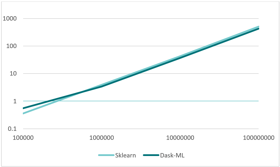
With data wrangling we saw that these libraries may not be useful unless we are working with huge datasets, as the computational cost of the functions is not that high. To see how these libraries work with functions with a higher computational cost, we fitted a clustering model with a randomly generated dataset with different numbers of entries: 100,000, 1,000,000, 10,000,000 and 100,000,000 entries.


100,000

1,000,000

10,000,000

100,000,000

Scikit-Learn

0.359504 s

3.916643 s

43.334999 s

502.258518 s

Dask-ML

0.550719 s

3.396780 s

37.125517 s

428.510227 s


Dask and Ray graphic


In this line plot we can see the benefits of using Dask when working with large datasets, and how it is of little help when we are not facing memory issues. We can see that the runtime improvement is logarithmic, so we can notice bigger improvements when working with larger datasets.


Conclusion


After our research, we found that these new libraries can be very useful when dealing with very large datasets or with tasks that require lots of computing resources. These libraries have been implemented to be easy to use for Pandas-friendly users, so you do not have to learn a whole new library from scratch.


What we must bear in mind is that these libraries should not be used unless they are needed, as they add some difficulty to the coding; and if we are working with small datasets, it would be overkill. As we saw with our tests, if we do not have any problems while running the code, we should keep using raw Pandas as it is the most efficient way to go.


Here at ClearPeaks, our team of specialists are always testing new developments and looking for solutions to your advanced analytics needs, so don’t hesitate to get in touch with us if there’s anything you think we can help you with!


Advanced Analytics Service

The post A Comparative Analysis of the Dask and Ray Libraries appeared first on ClearPeaks.
ODI Multiple Execution Units and their Advantages

$
0
0

In one of our customer projects, we needed to identify the part of an ODI (Oracle Data Integrator)-generated mapping query that ran for longer than expected and then fix it with the help of various options in Oracle SQL Query; but how could we do it in ODI?


One of the simplest and most effective options is to use hints or indexes. In ODI, it is only possible to apply Oracle hints or indexes on the overall SELECT at LKM (Load Knowledge Module) level, or on the final INSERT at IKM (Integration Knowledge Module) level. In these solutions, we may need to create separate DB objects in the background in order to make the query run faster.


In ODI12c, there is an option available to split the execution units in the same physical mapping layer. In this way we can separate the lines of SQL code (i.e. Sub SELECT/INLINE query) from the main pipeline, identified as a potential performance bottleneck. Splitting execution units (EUs) is not a new idea in ODI, and by default is taken care of by Groovy code while generating physical mapping. If there is only one target or the same physical/logical architecture with the same schema, then Groovy creates only one EU by sharing the same name as the target table, suffixing with _EU or simply <DataModelName>_UNIT.


If we separate the Sub-SELECT pipeline from the main flow as shown in demo example below, we can create a new EU of our own. This will allow us to bring in other EKM (Execution Knowledge Module) and LKM options to set, and also to execute the particular line of SQL code to run on a separate source or target or staging schema. Likewise, we can create N, the number of EUs in one single physical mapping. This is one of the major query optimisation features in ETL mapping performance using ODI.


Demo Example


In the following example, we have created a simple ETL flow by considering both source and target on the same database; Groovy treated it as one EU, US_ANALYTICS_UNIT, by default.


Demo Example ETL flow


Please note that this default physical mapping won’t allow the setting of a specific LKM (i.e. C$ temp table) at source level, as all are sharing the same physical/logical architecture.


When we check the same in Session Logs under Operator, we can see only one EU created.


Session logs


How to create a new EU


To make this demo use explicit LKMs or create separate EUs, we simply select the component at which point we would like to separate the flow from main pipeline and drag it outside the current execution unit so that it creates a new one automatically. Later, we can execute it in either a separate schema or just create a C$ temp work table so that we can apply the required temporary hints/indexes in LKM Options based on the LKM we use.


Before


Join Component


In this example, we have decided to separate the flow at the “JOIN” component, so we can do so by simply dragging it outside.


Here, we can see that the new component will be created as JOIN_AP, so when we click on this component, we can view LKM Selector and its corresponding Options in the Properties pane as shown below:


After


Join component After


Now when we execute this mapping, we can observe a new EU suffixed as _1, as shown below:


EU suffixed


This solution is more effective in large complex mappings, and we can clearly see the difference in performance. In this example, we created the demo with simple SCOTT schema tables and with small data.


Demo on Large Volumes of Data


Further to the above example, we will now show you a particular use case, dealing with large volumes of data based on a real project requirement. In this case, the data needs to be loaded into 2 separate targets in the logical mapping design (even though both logical targets point to the same physical table). The requirement and data integration logic is such that it requires different field criteria and insert/update logic in each of the targets.


Before the Changes


First, we tried to load a single EU as shown in the screenshot below, using default physical mapping (i.e. named Original):


load a single EU


We can see where the execution time for each pipeline took more than 2 hours:


execution time for each pipeline

After the Changes


Now, after splitting the EUs as shown below at the expression EXP_TGT in the new physical mapping (named Modified-1):


expression EXP_TGT


Compared with the previous run, execution time has been improved drastically, cutting the overall execution period by almost half, where the insert into the final target split has been loaded in no time at all. This example showcases how ETL performance can be twice as fast on average.


Below are the execution results after introducing the new EU:


execution results


Advantages:


  • Helps to achieve faster, optimised query performance across multiple targets based on Oracle recommendations.
  • Can be used to derive the inline query and fine-tune it without disturbing the main pipeline, especially in the case of reusable mappings and left outer joins. We are also consolidating the entire query in C$ and loading into multiple targets, based on requirements.
  • It is easy to transform the whole reusable mapping to merge inside the main mapping with the help of these EUs, dragging them outside.


Limitations:


  • Before making the changes, you must understand there won’t be any “undos” in ODI as per its basic UI design, so please ensure you have an original copy as mentioned in the point below.
  • It is preferable to create a new physical mapping that will create the EU for you before you start making modifications, rather than taking a backup copy of the entire mapping.


Here at ClearPeaks this is just one of the many solutions we’ve worked on in ODI, so if you’d like to learn more about how we can speed up your BI processes, just contact us!


The post ODI Multiple Execution Units and their Advantages appeared first on ClearPeaks.
Enhancing an AWS Data Platform with Airflow and Containers

$
0
0

Amazon Web Services (AWS) is the market-leading on-demand public cloud computing provider, getting more and more popular  year after year. AWS improves its services regularly and creates new ones every other month to tackle all sorts of workloads, so it’s hardly surprising that many companies, including a few of our customers, want to migrate their data platforms to AWS.


At ClearPeaks, we are experts on data platforms leveraging big data and cloud technologies, and we have a large team working on various AWS projects. And yes, it is true that this platform and its services offer a lot of possibilities, but sometimes it is easy to get lost among so many services to choose from.


In previous blog entries we have already offered some help in this regard, since in our previous entries we discussed how to build a batch big data analytics platform on AWS and also how to build a real-time analytics platform on AWS, in both cases using Snowflake as the data warehouse. In this blog article we are going one step further, to fill a couple of gaps that have traditionally existed on AWS data platforms, and that will, for sure, be of interest to anyone attempting to design a modern and capability-rich AWS data platform.


The first gap is in data ingestion: AWS has a plethora of services for doing all sorts of things with data already in AWS, but what options are there to bring data from outside ? As we will discuss below, there are services in AWS for bringing data from common types of sources, such as RDBMS, into AWS. But what happens when we are dealing with an uncommon source?


The second gap is orchestration: what options do we have if we need a tool or mechanism to allow us to schedule the execution of cross-service data pipelines in an organized and simple way?


Filling the Gaps


Regarding data ingestion for uncommon data sources, in AWS we can do it in different ways as we will discuss below, but in this blog we will explore and demonstrate a solution using Python code encapsuled in Docker, which pretty much allows us to do whatever we want for as long as we need and as often as we need.


Regarding orchestration, since our team is very active in AWS and we are in constant collaboration with their engineers, we were one of the first teams to test a new service in AWS  that specifically aims to fill this gap, Managed Workflows by Apache Airflow (MWAA). This new service gives us the possibility to use Airflow in AWS without the need to manage the underlying infrastructure.


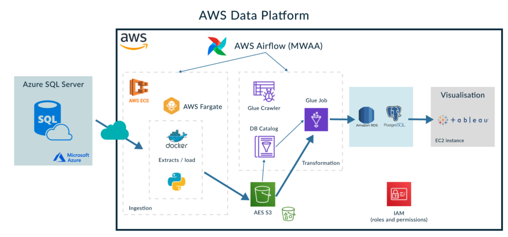
To illustrate the proposed solutions, we have built the platform shown below to address a simple use case:


AWS Data Platform


In this example, we are using Python and Docker to read data from an RDBMS into S3, make a simple transformation with Glue, store the transformed data in a PostgreSQL RDS and visualize it with Tableau; the ingestion and transformation steps are orchestrated by Airflow.


We are aware that an RDBMS is anything but uncommon! But bear with us since we just want to illustrate a simple example of building and using a custom connector to read from any type of source. For the sake of simplicity, we chose an RDBMS, but to make it a bit more challenging it’s from Azure; please note that you could use the same approach (of course with different Python code) for any other type of source.


Ingestion


As we have already noted, in some contexts where the data source is not traditional, connectors are not provided by AWS; so we may encounter some limitations when it comes to extracting and ingesting data from these sources. To overcome this limitation, leveraging a Docker container running Python code, we can connect to any type of data source by writing our own code and using the required set of libraries.


In our scenario, the Python code uses the “pyodbc” library to connect to the source database. In addition, we rely on the common “boto3” library (AWS SDK for Python) to manage AWS services. In our scenario, boto3 is used to store the extracted data in S3. Obviously, this code can be easily modified to connect to another type of database.


At the risk of explaining something you already know, we must emphasize that the development of the Python code and the creation of the Docker image is done in a local development environment running Ubuntu, where local tests can be executed.


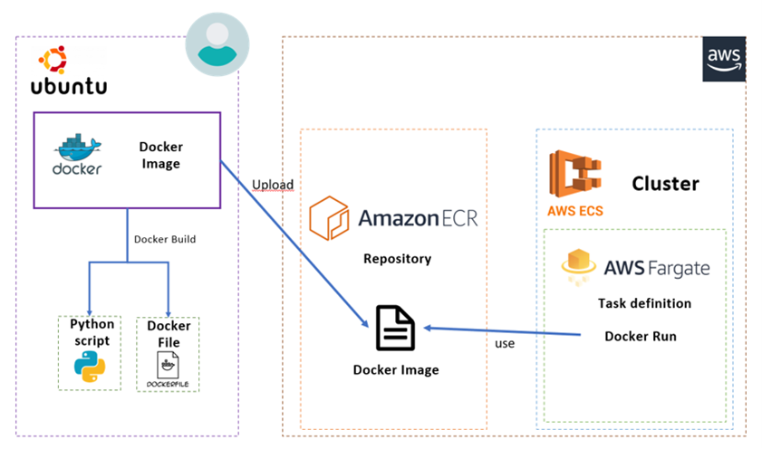
Our next step will be the preparation of the Dockerfile (the document that specifies the dependencies in order to execute the Python code correctly). Once both files are ready, the creation of the Docker image can be done by running a “docker build” command in our local development environment.  AWS provides a repository service for containers, AWS ECR, where we are going to push the created docker image. See the image below for more details:


Airflow AWS


AWS proposes several ways to run docker containers. Our approach uses AWS Fargate, which is a serverless compute engine for containers. We could have deployed the docker image in an EC2 instance, but as the ingestion process is only going to run once per day, AWS Fargate will cost less, and will also take care of the provision and management of the underlying servers.


We have chosen AWS ECS as the orchestration engine for the containers, which integrates well with Fargate and our use case (a single execution per day). We also tried AWS EKS, but it didn’t fit our scenario as it tries to keep the service up and available at all times, which was not a requirement for our use case.


If you want more information about how ECS and Fargate work together (and what the differences are) we recommend this blog article. 


Orchestration


Before the release of AWS MWAA, there were two approaches to orchestrate data pipelines in AWS: AWS Steps Functions, or using an event-based approach relying on AWS Lambda. Nevertheless, neither of these services met all the requirements expected of a data orchestration tool.


AWS MWAA is a managed service for Apache Airflow, which allows the deployment of the Airflow 2.0 version. AWS MWAA deploys and manages all aspects of an Apache Airflow cluster, including the scheduler, workers and web server. They are all highly available and can be scaled as necessary.


Regarding the sizing of the cluster, AWS MWAA only provides three flavours: small, medium, and large. By selecting one of the sizes, AWS dimensions all the components of the cluster accordingly, including DAG capacity, scheduler CPU, workers CPU, and webserver CPU. The cluster can also scale up to the maximum workers. For our use case, we chose the small one as we just need to schedule one pipeline.


The orchestration logic, i.e. the DAGs, developed in Python, are stored in S3 buckets; plugins and library requirement files are also synchronized with the Airflow cluster via S3.


The following image corresponds to the Airflow portal UI:


Airflow DAGs


One of the downsides of AWS MWAA is the fact that once deployed, the cluster cannot be turned off or stopped, so the minimum monthly cost of a cluster will be around $250.


In our project, we have used the operators to interact with AWS ECS and Glue services. Operators are pre-defined tasks, written by providers (AWS, Google, Snowflake, etc.)  and imported via libraries. Bear in mind that not all the tasks are available via operators, such as the execution of a Glue job. In this case, two other options are available: Hooks, which provides a high-level interface to the services, or we can use a Python operator and write the low-level code that connects to the API.


The following diagram represents the Airflow environment along with the files we developed and uploaded into S3 as part of our simple demonstration. Our DAG runs an ECSOperator and a PythonOperator. The ECSOperator controls the ECS service that runs the Docker container (on Fargate) that connects to the source (in this case the Azure DB) and loads the data into S3. The PythonOperator interacts with the Glue jobs via the API – it reads the data from S3 and loads it into the PostgreSQL RDS:


Managed workflow by Apache Airflow


Conclusion


Now let’s go over everything we have learned in this blog post, highlighting the important parts.


Through a simple example, we have presented an approach to ingest data into AWS from any type of source by leveraging Python and containers (via AWS ECS and Fargate), and we have also seen how the AWS MWAA service can be positioned as the main orchestration service ahead of other options such as AWS Step Functions.


We hope this article has been of help and interest to you. Here at ClearPeaks, our consultants have a wide experience with AWS and cloud technologies, so don’t hesitate to contact us if you’d like to know more about what we can do for you.


Big Data and Cloud Services blog banner

The post Enhancing an AWS Data Platform with Airflow and Containers appeared first on ClearPeaks.
Serverless Near Real-time Data Ingestion in BigQuery

$
0
0

Here at ClearPeaks we have been using Google Cloud Platform (GCP) in our customers’ projects for a while now, and a few months ago we published a blog article about a solution we had implemented for one of our customers in which we built a data warehouse on GCP with BigQuery. In that scenario, data was loaded weekly from a network share on our customer’s premises to GCP by a Python tool running on an on-prem VM. Every week the data was first loaded to Cloud Storage, then external tables were created in BigQuery pointing to the new data in Cloud Storage; lastly the data was loaded to the final partitioned tables in BigQuery from the external tables in an insert statement that also added a clustering column and some columns to monitor the loading procedure.


In this article, we will be describing another GCP data platform solution in a similar scenario that, while also leveraging Big Query, takes a different approach regarding how data is ingested compared to what we saw in our previous GCP blog. The most distinctive characteristics of the solution we are describing here are that it is fully serverless in that it uses only GCP services that are fully managed, and that it is capable of ingesting data into BigQuery in near real time.


Solution Overview


In the scenario described in this article, an upstream application dumps data periodically into an S3 bucket. There are multiple folders in S3, and each folder contains CSVs with a common schema, and a new CSV is added every few hours.


Input data in S3


Essentially, we want to load each folder in S3 into a table in BigQuery, and we need to load the new data landing in S3 into BigQuery as soon as possible. The loading procedure needs to make some minor in-row transformations – a few columns are added based on others, including a clustering column and columns to monitor the loading procedure. Moreover, the BigQuery tables are all partitioned by a date field. This combination of clustering and partitioning yields the best performance in queries.


We have designed and implemented a full serverless ingestion solution based on the one presented in this Google blog, but extended to be more robust. The solution consists of the following Google Cloud services: Google Cloud Storage, Google Cloud Transfer Service, Google BigQuery, Google Firestore, Google Cloud Functions, Google Pub/Sub, Google Cloud Scheduler and SendGrid Email API, the latter being a marketplace service. To avoid ending up with a lengthy article, we will not present all the services involved, so if you need more information about the services used please check the Google documentation.


What we will do now is to describe briefly how we have used each of the services in our solution before going into deeper tech details later:


  1. Cloud Storage: There are a number of buckets used for various reasons:
    • “Lake” bucket for the data files landing from S3; this bucket is split into folders like the one in S3.
    • Bucket for the configuration files.
    • Bucket to store the outcome of the periodic checks.
    • Bucket to store the deployed Google Cloud Functions.
    • Auxiliary buckets used internally during Google Cloud Function executions.
  2. Transfer Service: Different jobs, one for each folder, to bring data from the AWS S3 bucket to Google Cloud Storage.
  3. BigQuery: The final tables are in BigQuery; data needs to be loaded into these tables as soon as possible. Users will connect to BigQuery and query/extract data as they need, but instead of connecting directly to the tables with the data, they will connect via read-only views (which are actually in different GCP projects).
  4. Firestore: We use this NoSQL document store to track which files are loaded.
  5. Cloud Function: All the compute required by our ingestion solution is provided by Cloud Functions. There are two functions:
    • Streaming: used to stream data from Cloud Storage to Big Query.
    • Checking: used to validate the status of the last couple of months of data.
  6. Pub/Sub: The serverless GCP messaging broker is used to:
    • Re-trigger ingestion of files.
    • Trigger a periodic checking procedure.
  7. Cloud Scheduler: A periodic job to send a message to a Pub/Sub topic to trigger the checking procedure.
  8. SendGrid Email API: We use this marketplace service to send emails with the results of the periodic checking procedure.


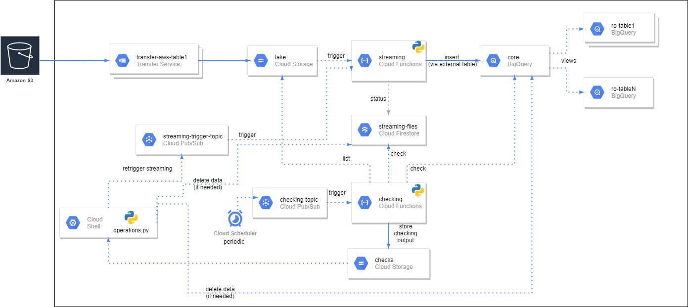
Service diagram and flow of our GCP serverless ingestion solution


Technical Details


Figure 2 above depicts the diagram and flow of the various services and the actions involved in our GCP serverless ingestion solution. Various Transfer Service jobs are created to transfer data from the S3 bucket to a Cloud Storage (CS) bucket. The transfer service jobs are scheduled to run periodically (every couple of hours), and each run only transfers the files that have been added recently and that do not already exist in the destination (our S3 files are immutable; they cannot be modified). We have one job per folder in S3 to gain better control over when the data of each folder is transferred.


A Cloud Function called streaming is created that will be triggered every time a file is created in CS. This streaming Cloud Function is implemented in Python and performs the following steps:

  • Check if the file is already ingested or if there is already a Function instance ingesting this file. A Google Cloud Storage trigger, while in principle this should not happen, can yield more than one Function Execution (see here for more information), so we have added a mechanism that, using Firestore, ensures each file is added only once.
  • If the file is not already ingested the Function instance:
    • Downloads the file locally (locally to the Function instance workspace).
    • Gets the number of lines in the file and its header.
    • Creates an external table pointing to the file in CS.
    • Inserts the data into the corresponding final BigQuery table. The insert statement does the required in-row transformation, e. adds the clustering field and the monitoring fields.
    • Deletes the external table in BigQuery and the local file.
  • The ingestion status is logged into Firestore. In Firestore, we also register the time spent on each of the steps, as well as other metadata such as the number of rows in the file.


A second Cloud Function called checking runs periodically and checks, for the current and previous month and for all the tables, that all files in Cloud Storage are also in BigQuery. A checking execution outputs, in Cloud Storage, a number of CSV files with the results of the check. In some cases, the checking function also carries out some minor fixes. More details on this later.


We have also created a script called operations.py that can be executed using Cloud Shell and that, given a CSV with links to CS files (which is what the checking function outputs), can:

  • Retrigger the streaming function (ingest data from CS to BigQuery) for a bunch of files. This also calls the streaming function, but in a second deployment that is triggered using Pub/Sub instead of CS triggers; essentially the Python code writes one message in Pub/Sub, for each file that needs to be ingested, with the location of the file.
  • Delete the related BigQuery data for the files. This mode must be operated with extreme care since deletion queries can be expensive.
  • Delete the related Firestore entries for the files.


Using operations.py can help us to deal with the outcome of the checking function. Below we can see a table that explains the various files that are output by the checking execution as well as the recommended action (DATE is the date when the checking function was run; NUM will be the number of lines of each file):


Output files of a checking function run and recommended actions


Note the final type of file in the above table: it will list files that are loaded in BigQuery but that appear as unsuccessful in Firestore. As you have seen above, the ingestion of a file itself is done by a run of a cloud function called streaming. An important thing to know about functions is that, while they are great, they time out after 9 minutes – which can be problematic in some cases.


In our case, most of the run time of a streaming function is spent on the insert statement, so a streaming function run may time out before the insert statement has completed. Luckily, BigQuery jobs are async anyway, so what the Python code actually does is submit the insert and wait for it to finish. If the function times out, only the wait is killed but not the insert, though the steps after the insert will not be executed – these steps basically delete the external table and update Firestore.


As mentioned in the table above, when executed, the checking function will fix these cases – when it detects that a file is in BigQuery but appears unsuccessful in Firestore, it will fix the Firestore entry, and also delete the external table. In any case, please note that the files that we receive are relatively small (less than 1GB) so on average a streaming function run takes around 5 minutes, so we do not often see this timeout situation (but we are ready for it).


Conclusion


In this article, we have presented a full serverless approach to ingest data into BigQuery in near real time. In our case, the input files are in AWS S3 and are brought to Cloud Storage using Google Transfer Service. Once a new file lands in Cloud Storage, it is loaded into BigQuery within a few minutes so users can query the data as soon as possible. The solution is quite generic and can be reused for other cases with minor modifications.


Here at ClearPeaks we are experts on building and operating data platforms in the main public clouds, including not only GCP but also AWS, Azure and Oracle Cloud. If you require expert brains and experienced hands for your cloud project, do not hesitate to contact us – we will be delighted to help you. Clouds are fun, and we love flying in them!


Big Data and Cloud Services blog banner

The post Serverless Near Real-time Data Ingestion in BigQuery appeared first on ClearPeaks.
Real-Time Streaming Analytics with Cloudera Data Flow and SQL Stream Builder

$
0
0

Real-time data processing is a critical aspect for most of today’s enterprises and organisations; data analytics teams are more and more often required to digest massive volumes of high-velocity data streams coming from multiple sources and unlock their value in real time in order to accelerate time-to-insight.


Whether it is about monitoring the status of some high-end machinery, the fluctuations in the stock market, or the amount of incoming connections to the organisations’ servers,  data pipelines should be built so that critical information is immediately detected, without the delay implied by classic ETL and batch jobs.


While both IT and Business agree on the need to equip their organisation (or their customer’s) with the latest state-of-the-art solutions, leveraging the latest and greatest available technologies, the burden of the implementation, the technical challenges and the possible scarcity of required skills always falls on IT. The general consensus, in fact, is that real-time streaming is expensive and hard to implement, and requires special resources and skills.


Luckily, this has changed drastically over the last few years: new technologies are being developed and released to make such solutions more affordable and easier to implement, turning actual real-time streaming analytics into a much more realistic target to pursue within your organisation.


One of the field leaders is, of course, Cloudera. Cloudera Data Flow (CDF) is the suite of services within the Cloudera Data Platform umbrella that unlocks the streaming capabilities that you need, both on-premise or in the cloud. Specifically, the combination of Kafka, NiFi (aka Cloudera Flow Management) and the recently released SQL Stream Builder (running on Flink, available with the Cloudera Stream Analytics package) allow data analytics teams to easily build robust real-time streaming pipelines, merely by using drag and drop interfaces and – wait for it – SQL queries!


Combining the information flowing from multiple Kafka clusters with master data stored in Hive, Impala, Kudu or even other external sources has never been easier, and anybody can do it, provided they know how to write SQL queries, without needing to specialise in any other technology, programming language or paradigm.


In this article, we will introduce CDF and its different modules, and dive deep into the SQL Stream Builder service, describing how it works, and why it would be a great addition to your tech stack. We will see how easy it is to use SQL Stream Builder to query a Kafka topic, join it with static tables from our data lake, apply time-based logics and aggregations in our queries, and write the results back to our CDP cluster or to a new Kafka topic in a matter of clicks! We will also see how easy it is to create Materialized Views, allowing other enterprise applications to access data in real time with the use of REST APIs. All of this from a simple web interface, with Single Sign On, in a secure, Kerberized environment!


CDF Overview


So, what exactly is CDF? To quote the definition from the Cloudera website, CDF is “a scalable, real-time streaming analytics platform”.​


Essentially, it is a collection of services to be installed beside your existing CDP cluster, or even independently, in order to create, monitor and manage streaming and real-time applications to ingest, move, modify, enrich or even consume your data.​


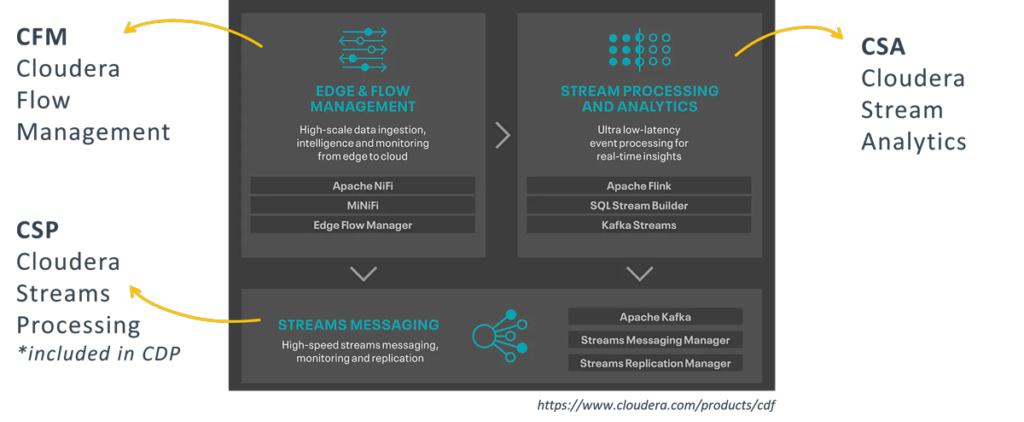
It is made up of 3 families of components, each covering a specific need.​ In the picture below, straight from the CDF website, we can see what these families are called, what services they include, and how they relate to the actual license packages that you need to acquire in order to run them.​


CDF components, as illustrated at https://www.cloudera.com/products/cdf

Figure 1: CDF components, as illustrated at https://www.cloudera.com/products/cdf


The first is Cloudera Flow Management, or CFM.​ CFM is used to “deliver real-time streaming data with no-code ingestion and management”.​


Practically, this translates to Apache NiFi – CFM is essentially NiFi, upgraded, packaged and integrated into the Cloudera stack, alongside other additional components which are tailored to work on edge nodes such as machines and sensors. It also includes a light version of NiFi called MiNiFi, and a monitoring application called Edge Flow Manager.​


The second package is called Cloudera Streams Messaging, initially branded as Cloudera Streams Processing (or CSP). The official definition says that it allows you to “buffer and scale massive volumes of data ingests to serve the real-time data needs of other enterprise and cloud applications”.​


In other words, it is basically Kafka, alongside two very useful new services for the management of the Kafka cluster:​

  • Streams Messaging Manager, or SMM, which is a very nice UI to monitor and manage the Kafka cluster and its topics.
  • Streams Replication Manager, or SRM, used to replicate topics across different clusters.​


Note that this component is actually included in the standard Cloudera Runtime for CDP Private Cloud: while it was initially branded as a separate module only, you are actually able to use it with your CDP license, without having to purchase an additional CDF license and install a new parcel.​


Finally, the last package – the one which we will focus on in the coming sections – is Cloudera Stream Analytics, or CSA.​ It is used to “empower real-time insights to improve detection and response to critical events that deliver valuable business outcomes”.​


Translated into practical terms, CSA is essentially Flink + SQL Stream Builder (SSB), and is Cloudera’s proposed solution for real-time analytics. As we said, in this article we will focus especially on SSB and test most of its capabilities.​


CSA and SQL Stream Builder


Before we describe SQL Stream Builder in detail, let’s look at why we should use CSA. As we said, Cloudera Stream Analytics is intended to “empower real-time insights”, and it includes Flink.


So, to start with, CSA offers all the Flink advantages, namely: event-driven applications, streaming analytics and continuous data pipelines,​ with high throughput and low latency,​ with the ability to write these results back to external databases and sinks.​


We can write applications to ingest real-time event streams and continuously produce and update results as events are consumed, materialising these results to files and databases on the fly; we can write pipelines that transform and enrich data while it is being moved from one system to another; and we can even connect reports and dashboards to consume all of this information with no additional delay due to batch loading or nightly ETL jobs.​


On top of this, CSA also includes SSB, which allows us to do all of this, and even more, without having to worry about how to develop a Flink application in the first place!​


The main functionality of SSB is to allow continuous SQL on unbounded data streams. Essentially, it is a SQL interface to Flink that allows us to run queries against streams, but also to join them with batch data from other sources, like Hive, Impala, Kudu or other JDBC connections (!!!).


SSB continuously processes the results of these queries to sinks of different types: for example, you can read from a Kafka topic, join the flow with lookup tables in Kudu, store the query results in Hive or redirect them to another Kafka topic, and so on.​ Of course, you can then connect to these targets with other applications to perform further analysis or visualisations of your data.​ With the Materialized View functionality, you can even create endpoints to easily consume this data from any application with a simple API call.


From a technical standpoint, SSB runs on Flink (when the queries are fired, they trigger stateful Flink jobs) and it is made up of 3 main components: the Streaming SQL Console, the SQL Stream Engine, and the Materialized View Engine.​


Hands-on Examples


Cluster Overview


Now, let’s get our hands dirty and play with CDF and SSB!


First of all, let’s take a look at what the Cloudera Manager portal looks like after installing the main CDF services:


Cloudera Manager portal with highlighted CDF services

Figure 2: Cloudera Manager portal with highlighted CDF services


Note that we are using the same Cloudera Manager instance for both the CDP and the CDF services. This, however, does not have to be the case: you can, in fact, have CDF in a separate cluster if required, as long as all necessary dependencies (for example, Zookeeper) are taken care of; the actual architecture will depend on the specific use cases and requirements.


SQL Stream Builder


When we navigate to the SSB service, the Streaming SQL Console is our landing page. We can immediately see the SQL pane where we will write our queries. At the top, we can see the name of the Flink job (randomly assigned), the Sink selector, and an Advanced Settings toggle. At the bottom, we have the Logs and the Results panes (in the latter, we will see the sampled results of all of our queries, no matter the Sink we selected).


The Streaming SQL Console in SQL Stream Builder

Figure 3: The Streaming SQL Console in SQL Stream Builder


On the left, we can see a navigation pane for all the main components of the tool;  we can see the Data Providers section, where we can have a look at the current Data Providers that we set up for our cluster: Kafka and Hive (automatically enabled by Cloudera Manager when installing SSB) and Kudu, which we added manually in a very straightforward process. Bear in mind that you can add more Kafka and Hive providers if necessary, and it is also possible to add Schema Registry and Custom providers, if required.


The Data Providers section

Figure 4: The Data Providers section


Back to the Console section, we move to the Tables tab, where we can see the list of available tables, depending on the Providers we configured. The first thing we notice is that we have different table types:


  • Hive catalog: tables coming from the Hive Data Provider, automatically detected and not editable.
  • Kudu catalog: tables coming from the Kudu Data Provider, automatically detected and not editable.
  • Kafka: tables representing the SQL interface to Kafka topics, to be created manually and editable.
  • Datagen/Faker: dummy data generators, specific to Flink DDL.


The Table tab in the Streaming SQL Console

Figure 5: The Table tab in the Streaming SQL Console


The other tabs – Functions, History and SQL Jobs – respectively allow us to define and manage UDFs, check out the history of all executed queries, and manage the SQL jobs that are currently running.


Example 1: Querying a Kafka Topic


In this first example, we are going to try to query a Kafka topic as if it was a normal table. To do so, we set up a Kafka table called rates, on top of a Kafka topic with the same name. We can see the wizard that allows us to do so in the picture below. Note how you also have a Kafka cluster, a data format, and a schema, which in our case we were able to detect automatically with the Detect Schema button, since our topic is already populated with data.


Wizard for the creation of a Kafka table

Figure 6: Wizard for the creation of a Kafka table


The topic is currently being filled by a small NiFi pipeline that continuously pulls data from a public API providing the live rates in USD of many currencies, including cryptos. Using Streams Messaging Manager (the new UI to monitor and manage the Kafka cluster) we can easily take a look at the content of the topic:


View of the Data Explorer in SMM, with a sample of messages in the ‘rates’ topic

Figure 7: View of the Data Explorer in SMM, with a sample of messages in the ‘rates’ topic


As we can see, all messages are in JSON format, with a schema that matches the one automatically detected by SSB.

Going back to the Compose tab, we now run our first query:


select * from rates 


As you can see, it is just a simple SQL query, selecting from rates as if it was a normal structured table. Since Sink is set to none, the result is simply displayed in the Results pane, and is continuously updated as more data flows into the topic.


Sampled results of the query on the ‘rates’ topic

Figure 8: Sampled results of the query on the ‘rates’ topic


Of course, we could also edit the query, just as we would do for any other SQL statement. For example, we could decide to select just a few of the original columns, apply a where condition, and so on.


If we look at the Logs tab, we can see how we effectively started a Flink job; this job is also visible in the Flink dashboard, to be monitored and managed just like any other Flink job. Furthermore, as we have already mentioned, all the SSB jobs can also be managed from the SQL Jobs tab in the SQL Console, alongside the History tab where we can see information about past executions.


Example 2: Joining Kafka with Kudu


We have seen above how to query unbounded data ingested in Kafka, a very cool feature of SSB. However, what is actually even cooler about this new tool is that it allows you to mix and match unbounded and bounded sources seamlessly.


In this new example, we join the live currency rates with some currency master data that we have in a pre-populated Kudu table.


select
	r.id,
	a.`symbol`,
    	a.`rank`,
	a.name,
	r.currencySymbol,
	r.type,
	r.rateUsd,
    	r.eventTimestamp,
	a.explorer
from ( select
      id,
      symbol,
      currencySymbol,
      type,
      CAST(rateUsd as DOUBLE) as rateUsd,
      CAST(eventTimestamp as TIMESTAMP) as eventTimestamp
      from rates
  ) r join `Kudu`.`default_database`.`impala::default.rate_assets_kudu` a
on r.id = a.id
where a.`rank` <=5


As you can see, this is nothing but SQL, yet we are joining a streaming source with a batch table! And we did not have to write a single line of code or worry about deploying any application!


Joining a Kafta topic with a Kudu table

Figure 9: Joining a Kafta topic with a Kudu table


Example 3: Storing Results to Hive


So far, we have only been displaying the results of our queries on the screen. However, you may wonder – can I store this somewhere? Luckily, the answer is yes: this is possible thanks to the Sink. In fact, we can select any of the tables defined in our Tables tab as Sink, provided (of course) that their schema matches the output of our query.


In this example, we run a query that is very similar to the previous one, but with 3 main differences:

  • The Sink is a previously created Parquet table.
  • the lookup data is in Hive and not in Kudu.
  • there is a “FOR SYSTEM_TIME AS OF PROCTIME()” clause in the Join statement.


select
	r.id,
	a.`symbol`,
    	a.`rank`,
	a.name,
	r.currencySymbol,
	r.type,
	r.rateUsd,
    	r.eventTimestamp,
	a.explorer
from ( select
      id,
      symbol,
      currencySymbol,
      type,
      CAST(rateUsd as DOUBLE) as rateUsd,
      CAST(eventTimestamp as TIMESTAMP) as eventTimestamp
      from rates
  ) r join `Hive`.`default`.`rate_assets_hive_txt` FOR SYSTEM_TIME AS OF PROCTIME() AS a
on r.id = a.id
where a.`rank` <=5;


While the change from Kudu to Hive is only to showcase another possible combination that SSB allows, the real difference in this case is in that extra clause in the join: that little piece of query is needed in order to allow Flink to effectively commit all the little partitions that it will create in the Hive table location. Without this, it would just keep adding data to a single partition without ever finalizing, and our Sink table would always be empty when queried.


Using a Parquet table as Sink for a real-time join query

Figure 10: Using a Parquet table as Sink for a real-time join query


If we query the Sink table while the job is running, we can see that it is actually being populated in real time by the output of our query:


Sample of the Parquet table being populated in real time

Figure 11: Sample of the Parquet table being populated in real time


Example 4: Applying a Window function


In the previous examples, we have run pure SQL queries, with the exception of the clause required to properly store the results back in HDFS. However, as mentioned, we can also use Flink-specific functions to perform certain time-based logics.


In this example, we use the WINDOW function, which allows us to group records and calculate aggregated metrics for a specific interval of time:


select
	id,
	symbol,
	currencySymbol,
	type,
	CAST(rateUsd as DOUBLE) as rateUsd,
	MIN(CAST(rateUsd as DOUBLE)) OVER last_interval AS min_rateUsd,
	MAX(CAST(rateUsd as DOUBLE)) OVER last_interval AS max_rateUsd,
	CAST(eventTimestamp as TIMESTAMP) as eventTimestamp
FROM rates where id = 'dogecoin'
WINDOW last_interval AS (
  PARTITION BY id
  ORDER BY eventTimestamp
  RANGE BETWEEN INTERVAL '1' MINUTE PRECEDING AND CURRENT ROW 
)


The above query will look very familiar to those of you who know how windowing functions work in SQL. We are partitioning the real-time rates by the currency ID, ordering by the record timestamp, and specifying an interval of 1 minute: essentially, for every currency, we are selecting the records that arrived in the previous minute and we are calculating the maximum and minimum rate in this interval. To help us understand the output, we also filter by one specific currency, in order to be able to see its evolution and notice how the aggregated measures change in time.


Results of a query using the Window function

Figure 12: Results of a query using the Window function


Note how both the minimum and maximum rate changed in a couple of seconds, according to the dogecoin rates received in the previous minute.


Example 5: Redirecting Results to a Kafka Topic


Not only we can store the results of our query in a table, but we can also redirect them to a new Kafka topic. We will now try to do so, using the same query as in the previous example.


First of all, we need to create a topic. In Streams Messaging Manager this is a very easy task: in the Topics section, we click on “Add New” and select the details for our topic. Note that in order for the Flink job to be able to effectively write the results there, we need to select the delete clean-up policy. We call the topic rates_window_sink.


Creating a new topic in SMM

Figure 13: Creating a new topic in SMM


Now that we have our topic, we need to create a Kafka table on top of it in SSB. Back to the Streaming SQL Console, we go to the Tables tab, and we add a new Kafka table. We assign a name, select the Kafka Cluster, select the topic we just created, our preferred format, and then we click on the Dynamic Schema checkbox. This will allow us to store messages with any schema in this table, without worrying about their consistency. However, notice how once we have done so, SSB tells us that this table can be only used as a Sink!


Creating a Kafka table for a Sink with Dynamic Schema

Figure 14: Creating a Kafka table for a Sink with Dynamic Schema


Once our table has been created, we run the previous Window query again, this time selecting our new Sink. Once the job has started, we go back to SMM to monitor our new topic, and we can see how data is effectively flowing in in real time as it is processed by the SSB query.


View of the Kafka Sink in SMM

Figure 15: View of the Kafka Sink in SMM


Example 6: Materialized View


Finally, in this last example, we will demonstrate the Materialized View functionality. Materialized Views can be thought of as snapshots of the query result that always contain the latest version of the data, represented by key. Their content is updated as the query runs, and is exposed through a REST endpoint that is associated to a key and can be called by any other application. For this example, we used the following query:


SELECT
	wizard,
	spell,
	CAST(COUNT(*) as INT) AS times_cast
FROM spells_cast
WHERE spell IN ('Expecto Patronum')
GROUP BY
	TUMBLE(PROCTIME(), INTERVAL '10' SECOND),
	wizard,
	spell


This query pulls data from a faker table, which is a type of connector available in Flink that allows us to create dummy data following certain rules. In our case, each row of the dummy dataset indicates a spell cast by a wizard . In our query, which uses another Flink function called TUMBLE, we want to count the number of times that a specific spell has been cast in the last 10 seconds by every wizard.


To create a materialized view for this query, we move to the pane of the Console tab, we select wizard as Primary Key, and we create a new API Key (if we did not have one already). As you can see below, there are more settings available. When we have finished, we click on “Apply Configurations”:


Creating a Materialized View

Figure 16: Creating a Materialized View


At this point, the “Add Query” button is enabled. This allows us to define API endpoints over the SQL query that we defined. Potentially, we can define multiple endpoints over the same result. We create one query by selecting all fields, and we click on “Save Changes”:


Creating an endpoint for a Materialized View

Figure 17: Creating an endpoint for a Materialized View


For every query we create, we get a URL endpoint. We can copy it and paste it in our browser to test our materialized view. If the job is running, we will obtain a JSON with the content of our view, as defined in our endpoint.


Result of our Materialized View endpoint

Figure 18: Result of our Materialized View endpoint


We are now free to take this endpoint and use it in any other application to access the results of our query in real time!


Conclusion


In this article, we have demonstrated how easy it is to build end-to-end stream applications, processing, storing and exposing real-time data without having to code, manage and maintain complex applications. All it took was a bit of SQL knowledge and the very user-friendly UIs of SQL Stream Builder.


We have also seen how useful some of the new CDF services are, particularly Streams Messaging Manager, a powerful solution to “cure the Kafka blindness”, allowing users to manage and monitor their Kafka cluster without having to struggle with Kerberos tickets and configuration files in an OS console.


In general, CDF has become a really comprehensive platform for all streaming needs. At ClearPeaks, we can proudly call ourselves CDF and CDP experts, so please contact us with any questions you might have or if you are interested in these or other Cloudera products. We will be more than happy to help you and guide you along your journey through real-time analytics, big data and advanced analytics!


If you want to see a practical demo of the examples above, head to our YouTube channel and watch a replay of our recent CoolTalks session on this topic. And do consider subscribing to our newsletter so that you don’t miss exciting updates!


Big Data and Cloud Services blog banner

The post Real-Time Streaming Analytics with Cloudera Data Flow and SQL Stream Builder appeared first on ClearPeaks.
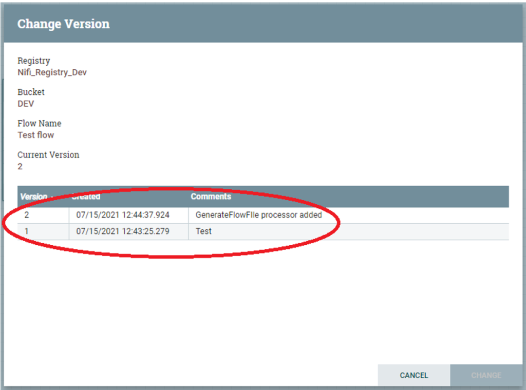
Power BI Goals

$
0
0

It is nothing new to say that data is currently one of the most important assets for the proper functioning of a company. However, it is not enough to know this data, study, and analyse it – companies must also set goals and challenges to achieve in the short-, medium- and long-term future to succeed.


Often, it is difficult to keep track of these targets. The lack of tools to automate their relationship with the datasets available and the required manual updates make this practice even more complex.


In the following article, we’ll learn about Microsoft Power BI Goals, a new feature from Microsoft that can address the aforementioned issues.


1. What is Power BI Goals?


Goals is a new feature recently released by Microsoft in Power BI Premium. Microsoft has defined it as follows: “Goals is a data-driven, collaborative, and adaptable way to measure key business metrics and goals built directly on top of Power BI. Goals enables teams to easily curate business metrics that matter most and aggregate them in a unified view.”


With this starting point, companies can measure their progress against their goals and work proactively, creating dedicated workspaces and scorecards to easily drive the impact of their KPIs.


2. How to Create a Power BI Goals Scorecard


For now, we can only access Goals features across the Power BI Service, where we can create a Premium Workspace to start developing our own Scorecard.


Creating a Scorecard is quite simple.


2.1 Steps to Create a Scorecard


First, we need to create an empty Scorecard in the Power BI Service, so we have to access it.


Once logged into the Power BI Service, the next step is going to the “Goals” view.


Power BI Goals Home Page

Figure 1: Power BI Goals Home Page


Once we’re inside this view, we can see our previously created Scorecards or create a new one by clicking on “New scorecard”. We can also check out sample Scorecards to test Goals functionalities and possibilities.


When we create a new Scorecard, a pop-up window appears to perform a general configuration:


Scorecard General Configuration

Figure 2: Scorecard General Configuration


As a premium feature, the Scorecard must be allocated in a premium workspace.


At this point, we can start setting up new goals to track our enterprise objectives by defining the objective’s name, setting its owner(s), current value, the target we want to achieve, start and due dates, and the status.


Goal Set-Up

Figure 3: Goal Set-Up


The status helps users to easily know if something is not started, on track, behind, overdone, at risk, or completed.


Goals can be hierarchy modeled with sub-goals tracking, with a maximum of 4 sub-levels which help us perform better deep-insight tracking.


Figure 4 - Goals Scorecard

Figure 4: Goals Scorecard


When we check-in new data updates across “Notes”, a Progress graph is automatically created, making it even easier to track the goal and detect irregularities or reassert a good pattern of data advancement.


2.2 Digging Deeper


Power BI Goals gives us the possibility to dig deeper inside our predefined targets by clicking on “Notes”.


Figure 5 - Goal Detai

Figure 5: Goal Details


In Goals “Bookcases”, we can also analyse the latest data updates, view their history, and add new ones.


3. Advanced Capabilities


To make Power BI Goals even more interesting, it has some other capabilities to transform Scorecards to obtain scalable, adaptable, flexible, and automated attributes.


3.1 Data-Driven Goals


For better data handling, Power BI Goals provides the capability to connect a Scorecard to one or more reports previously published in the Power BI Service. This feature automates data updates, thus reducing manual performance limitations.


To connect a goal to data from reports, we have to select the desired report when we are setting current or target values in the “Connect to Data” option. After the report is opened, we can filter tiles to get the required data value.


Report Data Connection

Figure 6: Report Data Connection


3.2 Status Rules


By default, goals’ statuses are set manually, but we can set up logical rules in a simple way to automate changes to improve users’ experience so that they can stay up-to-date and track the goals they have set.


Status-Rules

Figure 7: Status Rules


4. Goals on Mobile


Power BI also offers a first-class mobile experience, making it easy to perform updates and see the status of our key business metrics. Goals on Mobile has the same previously mentioned general capabilities to track goals from a Scorecard, with the addition of a soft, elegant, and interactive display.


phone-mock-gif Power BI

Figure 8: Goals on Mobile Gif


5. Next Steps and Limitations


Microsoft is constantly working on ambitious updates for the Power BI Goals feature and improving its user experience. Here are a few improvements the Microsoft team is working on:


  • Rollups: Users will be able to define rollups like sum, average, etc. to determine how sub-goals roll up to their goals.
  • Customisations: Goals will be provided with a rich set of formatting capabilities to customise Scorecards.
  • Power BI Desktop Goals: As we mentioned before, for now, Goals feature is only available in the Power BI Service and we can track them through the
    Power BI mobile app. In the next updates, it will also be possible to create Scorecards alongside other visuals in Power BI Desktop.
  • Power Automate Integration: It will be possible to automate business workflows based on triggers and actions derived from changes in goals.
  • Cascading of Goals: Users will be able to define a hierarchy based on Power BI data models, and it will automatically cascade their data-driven
    targets across the different levels.


However, there are some other capabilities not supported yet by Power BI Goals:


  • Row-level security (RLS) to restrict accessing data based on an authorisation context.
  • As we mentioned before, the maximum number of levels for sub-goals is four.


Conclusion


All in all, Power BI Goals is a new feature that can be used by any user, even by those without previous experience in Power BI. It offers an elegant and interactive organisational goals view of a company with perfect tracking possibilities.


In addition, it would be a very important improvement to the whole set if RLS is implemented in Power BI Goals to define roles that apply filters to restrict data at the row level. This feature could come with the Power BI Goals Desktop integration. Fingers crossed!


For a visual demo of Power BI Goals and how to use it, check out our YouTube video on the topic!


If you think Goals could meet your business needs, do not hesitate to contact us and we will be happy to help you.


In the meantime, do consider subscribing to our quarterly newsletter to stay updated on our latest news and insights!


Data Discovery and Visualizations service

The post Power BI Goals appeared first on ClearPeaks.
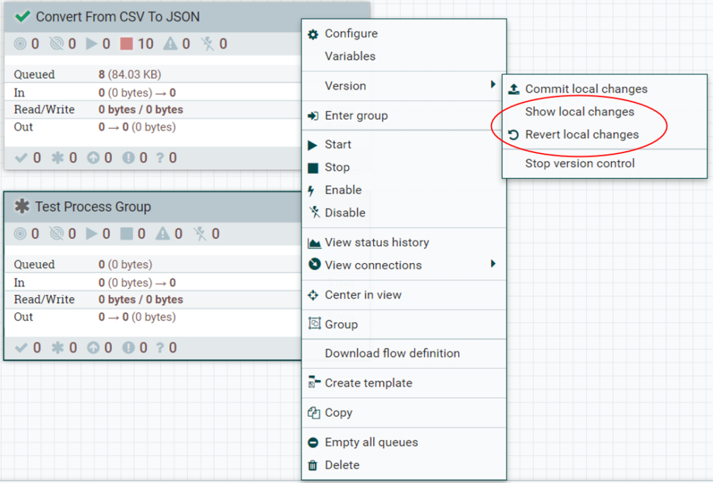

How Feature Engineering Trumps Algorithms

$
0
0

In the AI community we have recently seen a greater emphasis on moving from ‘Model Centric AI’ to ‘Data Centric AI’. Within the ‘Data Centric AI’ space there is an important  data science lifecycle component known as Feature Engineering, and in a world obsessed with modern algorithms, this component is often ignored or given a low priority in the pipeline. Feature engineering is more science than data, because domain knowledge and understanding the business problem form its essence.


introduction image


1. Methodology


In this article, we will focus on 3 different sets of feature engineering along with 3 different algorithms. We will test these 3 different methodologies on an electricity consumption dataset, and then compare the errors and conclude how feature engineering, when done right, can trump the choice of algorithms.


The algorithms used here are XGBoost, LightGBM, and GRU.


2. Dataset Description & Methodology


I will be using electricity consumption data at 15-minute intervals for a commercial building, which contains data from April 2017 till April 2018. This building has 3 meters (a main meter and 2 sub-meters), so we will predict 3 targets for each method.


The training set date range is from April 2017 till December 2017 and the test set from January 2018 till April 2018.


Since this is a forecasting problem, on the test set we used a weighted RMSE metric to evaluate forecasting errors. This metric gives greater weight to the nearer forecasted months and less weight to the predicted data further in the future.


Data for 1-Apr-2017 for a complete day

Figure 1: Data for 1-Apr-2017 for a complete day


3. Feature Engineering#1 with XGBoost


Monthly power consumption

          Figure 2: Power consumption on 2-Apr-2017 (Sunday)                                                    Figure 3: Monthly power consumption                    


A few important points to note about the data which will help us to make new features are:

  • There is a sudden spike in consumption from 6 AM to 6 PM. We could build a feature like ‘working hours’ (Figure 1).
  • On weekends (Sundays) power consumption is relatively low compared to weekdays, so we will build features for days as well (Figure 2).
  • Power consumption is high in the June-August and November-January periods, whereas consumption is lower in the remaining months in the main meter readings (Figure 3). We can construct 2 more features like ‘season’ and ‘months’.


After incorporating these features, we took the training set and we trained the hyper-tuned XGBoost algorithm. Evaluation results for the test set show:


Main Meter Error

Sub-meter#1 Error

Sub-meter#2 Error

Overall Avg. Error

30.4

15.3

33.2

26.3


Sample Predictions for 1-Apr-2017

Figure 4: Sample Predictions for 1-Apr-2017


4. Feature Engineering#2 with LightGBM


Now we will explore what our results would be if we used a different set of features and a different algorithm.

  • Construct quarter of the hour (0–3), hour of the day (0–23), day of the month, day of the week, month start and month end indicators for each row. Additionally, we could roll up the target value for each of the above features based on its hierarchy. This would give summarised target values for each data point.


Ex: building_number_dayofweek_hourofday_quarterofhour_mean for 1-Apr-2017 23:00 would be derived by taking the average of all target values which have building_number=1, dayofweek=5, hourofday=23, quarterofhour=0.


  • The above features can also be converted to cyclical features using sine and cosine transformations. This is done as it can preserve information such as the 23rd hour and 0th hour being close to each other.


After incorporating the aforementioned features, we took the training set and we trained the hyper-tuned LightGBM algorithm. Evaluation results for the test set show:


Main Meter Error

Sub-meter#1 Error

Sub-meter#2 Error

Overall Avg. Error

29

26

42.1

32.3


5. Feature Engineering#3 with GRU


In this final section, I will experiment with GRU (Gated Recurrent Unit), a special type of Recurrent Neural Network, part of Deep Learning algorithms, especially used for time-series data.


  • Construct a corporate feature which takes binary values. For working hours (8 AM to 8 PM) this will be set as 1 and for the rest it will be set as 0.
  • Construct day of week feature in the form of One Hot Encoding.


I tried different GRU model configurations: I have tried both training individual models for each meter of each building, and a generalised building-specific model too. I found that the generalised building-wise model, which predicted all the three-meter readings simultaneously, worked better than individual models for each meter.


Neural Network architecture used

Figure 5: Neural Network architecture used


After incorporating the mentioned features, we took the training set and we trained our neural network for 35 epochs. Evaluation results for the test set show:


Main Meter Error

Sub-meter#1 Error

Sub-meter#2 Error

Overall Avg. Error

32.7

25.5

31.6

29.9


Conclusion


This concludes my experiment for different sets of features used with different types of ML/DL models. We can clearly see that feature engineering set#1 with XGBoost gave the best predictions out of the 3 sets. Set#2 contains more mathematically-inclined features, but somehow fails to give the lowest error. In set#1, features are more diverse, intuitive and domain-specific.


Sometimes we need to construct features which are simpler, but can explain as much variance in data as possible, which help the model to learn more efficiently. Some features may make mathematical sense, as seen in set#2, but may not be as powerful as you’d expect. It’s trial and error: try different combinations of features with different ML/DL techniques, then settle for the one which gives you the best accuracy or lowest error.


We would really like to discuss the enterprise solutions and services that we can offer to help you reap the benefits of data science in your business. Send us an email and find out how our expertise can help you in your advanced analytics journey!


Advanced Analytics Service

The post How Feature Engineering Trumps Algorithms appeared first on ClearPeaks.
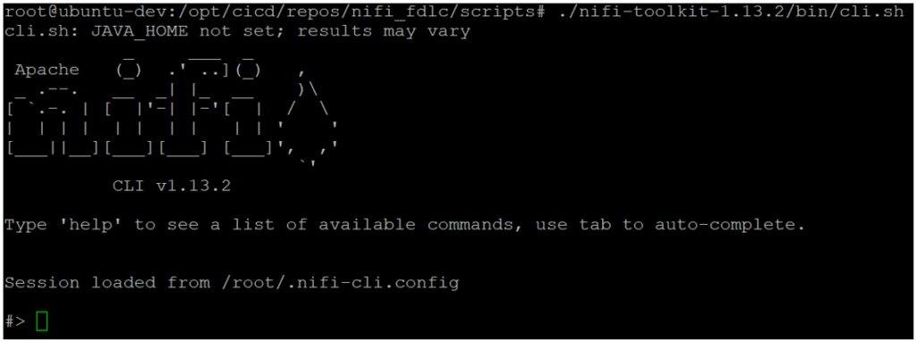
Integrating Apache MiNiFi with Apache NiFi for Collecting Data from the Edge

$
0
0

Business Intelligence (BI) is now a very well-known term among decision-makers. We could say that the concepts, methodologies, and paradigms behind the term are popping up almost every day, and these new additions are not only related to technology, but also to a way of thinking and to the agreements between people working together on projects. Bearing this in mind, there is one term which is, we could say, complementary to BI, and that is Operational Intelligence (OI).
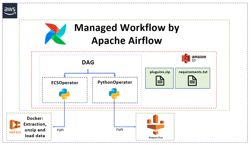
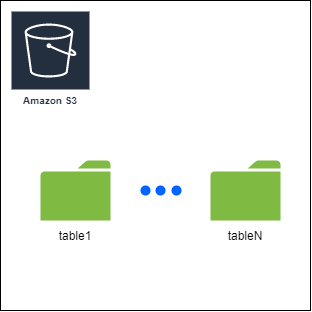
 

Operational Intelligence is an ecosystem of business rules, technology and concepts which can answer the question “What is going on right now, at this very moment?”, while BI, on the contrary, answers the question “What happened before, in the past?” in order to obtain insights into the future.


To be able to answer this question, OI needs to use fast technology which can ingest data from the very place where it is generated (data on the edge) and serve that data for consumption in a real-time or near real-time manner – the data is then processed in streams and time windows. There are also some general terms emerging from OI which are very popular today: Internet Of Things (IoT), Smart Cities, and Smart Industry.


In this article, we will demonstrate how to build an IoT ecosystem for collecting data from the edge in near real time, using Apache NiFi, Mosquitto message broker and Apache MiNiFi running on a Raspberry Pi 3B+. So let’s get started with a short introduction to these technologies.


Apache NiFi is a robust and scalable solution to automate data movement and transformation across various systems. Alongside Apache NiFi, we will use Apache MiNiFi:  a subproject of Apache NiFi and a lightweight version of it, which means most of the processors are not preloaded and there are some internal differences that make it more convenient for running on the edge, like in embedded computers close to the data source  (sensors, signal processors, etc.). Both NiFi and MiNiFi are offered by Cloudera as part of Cloudera Data Flow, but for this article we will use open-source versions.


For our demonstration, MiNiFi is running on a Raspberry Pi model 3B+  and acting as a data gateway, i.e. the point where data is collected and routed to a higher domain for further processing. Note that in this article we are demonstrating data collection, but not further processing.


We are also using Mosquitto message broker, a lightweight service to send messages securely from one point to another following a publish/subscribe model, ensuring the messages are not lost. Mosquitto is an implementation of the MQTT protocol, which is used for communication on low bandwidth networks and where resource consumption needs to be low, like embedded computers, phones or microcontrollers.


1. Demo Architecture


Our demo environment consists of the components represented in the picture below:


Demo architecture

Figure 1: Demo architecture


On the right we can see the data source (a radio tower belonging to an imaginary telecommunications company). In that tower, signals are processed and captured, and from these signals data about phone calls is generated, as well as data from SMS traffic and from people surfing the internet.


For this article, we will simulate SMS traffic data on the radio tower, and we will capture that data using the previously mentioned technologies. SMS traffic data is generated by a JSON data generator running on the Raspberry PI microcomputer; this simulates operational (OT) data generated by hardware on real telecommunications towers. The JSON data is then forwarded to the Mosquitto message broker which forwards the messages on to the MiNiFi agent. This agent is the real data mediator: it sends the received data to the NiFi instance running on a Linux Virtual Machine (VM) on a server in the same network using Site-to-Site protocol (in a real scenario, the NiFi instance would be on a separate remote server, in a different geographical location).


On that server, represented on the left of the picture, data can be further processed and prepared for storing into various analytics storages or time-series databases for real-time analysis and dashboarding, or even for alerting purposes. Note that in real life there would also be some sort of streaming platform, such as Kafka, for buffering the messages from multiple towers. However, to simplify our demonstration, we are putting everything in the same location, without a streaming platform in the middle.


2. Preparing the Services


Before the actual demonstration of streaming data from the Raspberry Pi to the NiFi instance, we will go through the installation and configuration steps for the services. After these steps, we will demonstrate how to integrate Apache MiNiFi and NiFi service with the rest of the components: Mosquitto message broker and the JSON data generator.


2.1. Installing and Configuring Apache NiFi


Apache NiFi can be downloaded from the official project website in the form of binary files. At the time of writing, the latest stable version is 1.14.0. After the download, the NiFi files can be unpacked and installed in the desired folder on the Linux VM, which we will refer to as $NIFI_HOME. In the installation folder there are other important folders, like $NIFI_HOME/bin and $NIFI_HOME/conf. An important requirement to run NiFi is to have Java version 1.8+, and to set the Java home path as an environment variable; to do so, use the following commands:


[user@host]# apt-get install openjdk-8-jdk
[user@host]#  nano /etc/environment # set $JAVA_HOME=”path/to/jvm/installation/folder”
[user@host]#  source /etc/environment
[user@host]#  java -version #check installed Java version


To configure NiFi to start on the desired localhost port, edit the file nifi.properties in  $NIFI_HOME/conf and set the following lines under the section #web properties, as shown below:


nifi.web.http.host=0.0.0.0
nifi.web.http.port=8081 


To ensure that NiFi is able to receive the data from another NiFi or MiNiFi instance using the Site-to-Site protocol, change the following lines in the same file:


# Site to Site properties
nifi.remote.input.host=
nifi.remote.input.secure=false
nifi.remote.input.socket.port=1026
nifi.remote.input.http.enabled=true
nifi.remote.input.http.transaction.ttl=30 sec
nifi.remote.contents.cache.expiration=30 secs 


After this, we can go to the folder $NIFI_HOME/bin and install NiFi as a service on the Linux VM; to do so, use the following command:


[user@host]# ./nifi.sh install nifi 


After this command, NiFi is installed on the Linux VM as a service named “nifi”. We can now start NiFi and check that everything has gone well by opening the URL http://localhost:8081/nifi in our web browser. If the NiFi UI is shown, NiFi is ready for flow development.


To check the status or to start/stop the NiFi service, use the following commands:


[user@host]#  service nifi status
[user@host]#  service nifi start
[user@host]#  service nifi stop


2.2. Installing Apache MiNiFi


Apache MiNiFi is installed on the Raspberry Pi microcomputer. The binaries can be downloaded from the official project website. At the time of writing, the latest stable version is 1.14.0. After the download, files can be unpacked in the desired installation folder, which we will refer to as $MINIFI_HOME. In the installation folder there are also other important folders such as $MINIFI_HOME/bin and $MINIFI_HOME/conf. The requirements to have Java 1.8+ installed and the Java home path set as an environment variable also apply to MiNiFi, and we can do so using the same commands as shown in the previous step.


To install MiNiFi as a service on the Raspberry Pi, open the folder $MINIFI_HOME/bin and use the following command:


[user@host]# ./minifi.sh install minifi


After the service has been installed, we can use the same commands as for NiFi to check the status of the MiNiFi service, or to start/stop it:


[user@host]#  service minifi status
[user@host]#  service minifi start
[user@host]#  service minifi stop


The MiNiFi agent is now ready to use, but we are not going to start it yet as we first need to develop the flow which will run on it.


Generally, there are two ways of developing MiNiFi flows: the first one is to manually create a YAML file, which is basically the flow configuration and the MiNiFi instance configuration used at the MiNiFi agent start-up. To create such a YAML file manually is cumbersome, so it is usually better to pick the second option, and that is to develop the flow using the NiFi UI and to save it as a template in XML format. After that, the MiNiFi toolkit can be used to convert the template XML file into a configuration YAML file which can be deployed on the MiNiFi instance on the Raspberry Pi. This YAML file is basically the definition of the flow, which will start automatically after starting the MiNiFi agent.


2.3. Installing Mosquitto Broker and the JSON Generator


To handle the generated JSON data, we will install the Mosquitto message broker on the Raspberry Pi. To do so, we can use a standard Linux package manager to fetch the latest stable version of the broker from the internet and to install it (at the time of writing, the latest version of Mosquitto message broker is 3.1.1 and the MQTT protocol is version 3.1). We use the following command:


[user@host]#  apt-get install mosquitto


After the installation, the Mosquitto service starts automatically and listens on port 1883 for incoming messages.


To simulate SMS traffic data, we use the JSON data generator, which can be downloaded from the GitHub repository. After unpacking the generator files in the desired installation folder, we use the JAR file “json-data-generator-1.4.0.jar” to run the generator.


Before running the generator, we must create two configuration files to define the details of the stream simulation, including what data to generate and how fast. Some configuration file examples are located in the ./conf folder, which is where we put the two configuration files for our demo.


The first configuration file defines the type of data that will be generated and its frequency. This file looks like the one shown below:


{
  "eventFrequency": 40,
  "varyEventFrequency": true,
  "repeatWorkflow": true,
  "timeBetweenRepeat": 200,
  "varyRepeatFrequency": true,
  "steps": [
    {
      "config": [
        {
          "SendDateTime": "nowTimestamp()",
          "SMSChannelId": "random(260987,261000,261383,90922,202007,203417)",
          "NetworkId": "random(540,5663,847,2502,4822,5664,1213,1428,2450,3204)",
          "GatewayId": "random(13,15,29,92,94,96,136,138,163,170,172,180)",
          "SMSCount": "random(1,2)"
        }
      ],
      "duration": 0
    }
  ]
}


In this configuration file we have some JSON fields defining the data generator workflow:


  • eventFrequency – the time in milliseconds between the steps (our generator has only one step)
  • varyEventFrequency – if true, a random amount (between 0 and half the eventFrequency) of time will be added/subtracted to the eventFrequency
  • repeatWorkflow – if true, the workflow will repeat after it finishes
  • timeBetweenRepeat – the time in milliseconds to wait before the workflow is restarted
  • varyRepeatFrequency – if true, a random amount (between 0 and half the eventFrequency) of time will be added/subtracted to the timeBewteenRepeat
  • steps – the data that will be generated in the form of a one-line JSON string; for every field in the JSON string a random value will be picked and the step will run only once, defined by the field “duration” with value 0


The second file serves as definition of the workflow name and of the data sink. The configuration file looks like this:


{
  "workflows": [
    {
      "workflowName": "SMSTraffic",
      "workflowFilename": "sms_traffic_generator.json"
    }
  ],
  "producers": [
    {
      "type": "mqtt",
      "broker.server": "tcp://localhost",
      "broker.port": 1883,
      "topic": "/rpi/sensors/basetower1",
      "clientId": "BaseTower1",
      "qos": 2
    }
  ]
}


The field “workflowName” is an internal field of the JSON generator and it is arbitrary, just to give a name to the workflow. The next field is “workflowFilename”, which refers to the first configuration file, where we defined what data will be generated and how fast. The rest of the fields define the remaining details of the data sink:


  • type – type of sink: in our case, Mosquitto broker which implements the MQTT protocol
  • server – the hostname or IP address of the machine where Mosquitto broker is running
  • port – the Mosquitto broker port
  • topic – the topic where the data is sent
  • clientId – arbitrary name of the client which sends the data
  • qos – Quality of Service, an important aspect of the MQTT protocol which defines the quality of message transfer. In our case it is level 2, which means every message will be transferred exactly once and is guaranteed not to be lost


With this configuration, the JSON data generator will send JSON strings like the one represented below to the Mosquitto message broker every 200 milliseconds; since there is only one step in the workflow, the “eventFrequency” field is ignored:


{"SendDateTime":"2021-09-23T11:57:22.882Z","SMSChannelId":289109,"NetworkId":3965,"GatewayId":1594,"SMSCount":2}


3. Preparing the Flows for NiFi and MiNiFi


Before starting the MiNiFi agent and generating the SMS traffic data, we need to develop the NiFi and MiNiFi flows which will handle the data stream. As we said earlier, we will develop the MiNiFi flow using NiFi running on a Linux VM because it is the easiest way.


In the picture below there are two process groups: on the right, we can see the process group that will run on the MiNiFi agent on the Raspberry Pi, collecting data from the Mosquitto message broker. On the left, we can see the process group that will run on NiFi on the Linux VM: it consists of one simple flow containing one input port and one dummy process group in which logic for further processing can be developed (like routing the data to multiple destinations, filtering it, or storing it to the final storage like time-series databases). The input port listens for data coming from other NiFi or MiNiFi instances on port 1026, as configured before. In our case, data will be coming from MiNiFi running on the Raspberry Pi.


NiFi and MiNiFi flows

Figure 2: NiFi and MiNiFi flows


Once again, note that the process group on the right is developed in NiFi, but will run on the MiNiFi agent, not on the NiFi instance.


3.1 The MiNiFi Flow


The picture below depicts the MiNiFi flow. Before data is sent to the NiFi instance, every flowfile is enriched with some additional attributes like timestamp, clientId, agent and flow version.


MiNiFi flow

Figure 3: MiNiFi flow


The first processor in the pipeline is ConsumeMQTT, which pulls JSON data from the Mosquitto message broker. The properties of the processor are shown in the pictures below. The processor connects to the localhost Mosquitto service, running on port 1883.


ConsumeMQTT properties

Figure 4: ConsumeMQTT properties (1/2)


ConsumeMQTT properties

Figure 5: ConsumeMQTT properties (2/2)


The topic to which the processor is subscribed is located on the path “/rpi/sensors” and it is called “basetower1”. Here we are using the wildcard “#” to receive data from all the topics on that path, although we have just one topic. Quality of service is set to level 2 to guarantee that messages will not be lost and will be delivered exactly once. To ensure this, the processor uses a queue into which it buffers the messages if the processor’s run schedule is behind the rate messages are coming in.


The next processor in the pipeline is UpdateAttribute, which adds some additional flowfile attributes to every message. This is an example of how the data stream can be enriched with some arbitrary data that has meaning for us. In the picture below, we can see the details of the additional attributes: agent – name of the MiNiFi agent, clientId – name of the radio tower, timestamp – date and time when a message entered MiNiFI flow and version – the MiNiFi flow version.


Attributes added to flowfiles

Figure 6: Attributes added to flowfiles


4. Configuring MiNiFi Agent


As mentioned earlier, we need to convert the NiFi flow template, developed in NiFi, to a YAML file that the MiNiFi agent will use as the flow configuration. To do so, we use MiNiFi Toolkit v1.14.0 and the script called “config.sh”, located in the ./bin folder of the toolkit installation:


[user@host]# ./bin/config.sh transform /path/to/template.xml /output/path/config.yml


The first argument of the script is the path to the exported NiFi flow template in XML; the second argument is the path to which the script saves the converted YAML file. Note that the filename is “config.yml” and it must not be changed.


After converting it, we copy the YAML file into the $MINIFI_HOME/conf folder and replace the old “config.yml” file. This is the file that the MiNiFi agent uses for initial flow and instance configuration.


Before starting the MiNiFi agent, we open the “config.yml” file and add some additional properties, which are crucial for communication between MiNiFi and NiFi. As we configured NiFi running on a Linux VM with Site-to-Site port 1026, we need to do the same in the configuration of the MiNiFi agent. We add the port and the hostname to which MiNiFi is sending data, right under the field “Input Ports”, as shown below:


  Input Ports:
  - id: AUTOGENERATED_NIFI_PORT_ID_HERE
    name: MiNiFi-input
    comment: ''
    max concurrent tasks: 1
    use compression: false
    Properties:
        Port: 1026      
        Host Name: 192.168.1.9 #ip address of the Linux VM running on separate server


5. Starting the Data Stream


After completing the necessary setup, we can finally start the JSON data generator and the MiNiFi agent to stream the data into NiFi. To start the MiNiFi agent, use the following command on the Raspberry Pi:


 [user@host]# service minifi start


After a few minutes, we use the “minifi.sh” script from the $MINIFI_HOME/bin folder to check the MiNiFi instance status, confirming that everything is running correctly:


[user@host]# minifi.sh flowStatus instance:health,stats,bulletins


The response from the script shows that everything is running smoothly, without any error bulletin:


Status of MiNiFi instance

Figure 7: Status of MiNiFi instance


After successfully starting the MiNiFi agent, we also start the JSON data generator on the Raspberry Pi, using the following command:


[user@host]# java -jar json-data-generator-1.4.0.jar sms_traffic_config.json


The generator starts to produce JSON messages and sends them to Mosquitto message broker, as shown in the picture below:


JSON data generator running

Figure 8: JSON data generator running


Immediately after starting the JSON generator, we can see the messages coming into the Input Port in NiFi.


JSON flowfiles collected by NiFi

Figure 9: JSON flowfiles collected by NiFi


We will now list the relationship to inspect the contents of the flowfiles and flowfile attributes, as generated by the MiNiFi flow. As we can see in the picture below, the payload of every flowfile is the JSON string message generated by the JSON data generator on the Raspberry Pi. Note that it also includes the timestamp (field “SendDateTime”), to simulate when the event occurred in the source (i.e. in the radio tower).


JSON message string collected by NiFi

Figure 10: JSON message string collected by NiFi


In the NiFi flow (on the Linux VM server), we can also add an UpdateAttribute processor to capture the timestamp when the flowfiles actually entered the flow.


Message timestamp in NiFi

Figure 11: Message timestamp in NiFi


Now we have both the timestamp when the message was created in the simulated radio tower (SendDateTime field: 2021-09-23T15:09:12.740 Z), and the timestamp when the message entered the first processor in NiFi (nifi_timestamp attribute: 2021/09/23 15:09:13.318Z). This is a further example of enriching the data using Apache NiFi: we can add arbitrary flowfile attributes with some information or values that can be generated dynamically as data flows through the pipeline.


Conclusion


This article shows how we can leverage Apache NiFi and MiNiFi in combination with Mosquitto message broker and a JSON data generator to collect data from a simulated radio communications tower in near real time. The radio tower was simulated using a JSON data generator and a Raspberry Pi microcomputer, which was also where the MiNiFi agent was running: today, this paradigm is called Edge Computing.


With these tools, data can be streamed and processed in near real time, which is crucial to monitoring events and processes exactly when they are happening. This enables fast responses to some critical events, to establish predictive maintenance, or to carry out system optimisations at the right time.


At ClearPeaks we are experts on solutions like the one demonstrated in this article. If you have interesting use cases or any questions related to data streaming, simply contact us, and we will be happy to discuss them with you!


Big Data and Cloud Services blog banner

The post Integrating Apache MiNiFi with Apache NiFi for Collecting Data from the Edge appeared first on ClearPeaks.